Advanced Lane Finding Project
The goals / steps of this project are the following:
- Compute the camera calibration matrix and distortion coefficients given a set of chessboard images.
- Apply a distortion correction to raw images.
- Use color transforms, gradients, etc., to create a thresholded binary image.
- Apply a perspective transform to rectify binary image ("birds-eye view").
- Detect lane pixels and fit to find the lane boundary.
- Determine the curvature of the lane and vehicle position with respect to center.
- Warp the detected lane boundaries back onto the original image.
- Output visual display of the lane boundaries and numerical estimation of lane curvature and vehicle position.
Rubric Points
Here I will consider the rubric points individually and describe how I addressed each point in my implementation.
Writeup / README
1. Provide a Writeup / README that includes all the rubric points and how you addressed each one. You can submit your writeup as markdown or pdf. Here is a template writeup for this project you can use as a guide and a starting point.
You're reading it! Note that below I will refer to the different code cells in my IPython notebook where I have made each part separately. The pipeline was later on summarized as functions, which can be seen in code cells 16-18 and 22. If you only want to run the pipeline these cells and the 1st cell needs to be run (note that this assumes that you have saved the calibration file).
Camera Calibration
1. Briefly state how you computed the camera matrix and distortion coefficients. Provide an example of a distortion corrected calibration image.
The code for this step is contained in the second and third code cell of the IPython notebook located in "AdvancedLaneLines.ipynb".
In the second code cell I start by preparing "object points", which will be the (x, y, z) coordinates of the chessboard corners in the world. Here I am assuming the chessboard is fixed on the (x, y) plane at z=0, such that the object points are the same for each calibration image. Thus, objp is just a replicated array of coordinates, and objpoints will be appended with a copy of it every time I successfully detect all chessboard corners in a test image. imgpoints will be appended with the (x, y) pixel position of each of the corners in the image plane with each successful chessboard detection.
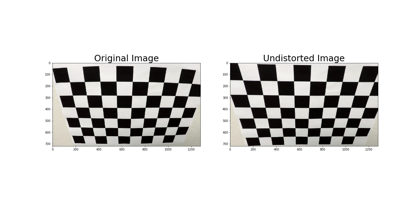
In the third code cell I then used the output objpoints and imgpoints to compute the camera calibration and distortion coefficients using the cv2.calibrateCamera() function. I applied this distortion correction to one of the calibration images using the cv2.undistort() function and obtained this result:
Pipeline (single images)
1. Provide an example of a distortion-corrected image.
This step can be seen in code cell 4 of my notebook. In this step, I applied the distortion correction (saved from camera calibration) to one of the test images like this one:

2. Describe how (and identify where in your code) you used color transforms, gradients or other methods to create a thresholded binary image. Provide an example of a binary image result.
In code cell 6 and 7 I used a combination of color and gradient thresholds to generate a binary image.
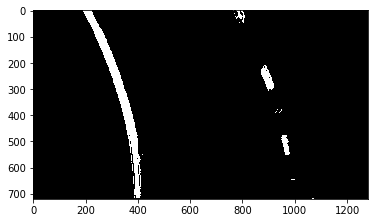
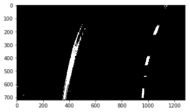
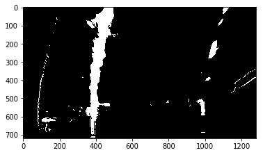
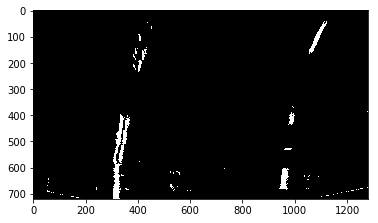
I found what color transformations and thresholdings to use by looking at the different output images for all test images. I chose to combine the best methods to find yellow lines with the best for detecting white lines. I also needed to take into consideration different thresholds to find the images independent on if the road was dark or light colored and if there was some shadows or other difficulties on the road.
To detect yellow lane markings I used the pixels which were either present in all of:
- S channel in HLS image (threshold 2)
- V channel in Luv image (threshold 1)
- x sobel of the R channel of RGB image
or in all of:
- S channel in HLS image (threshold 1)
- V channel in HSV image (threshold 1)
- V channel in Luv image (threshold 2)
To detect white lane markings I used the pixels which were either present in all of the following:
- L channel of HLS image (threshold 2)
- V channel of HSV image (threshold 2)
- x sobel of the R channel of RGB image
or in:
- L channel of HLS image (threshold 1)
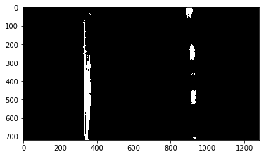
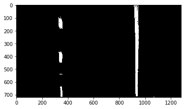
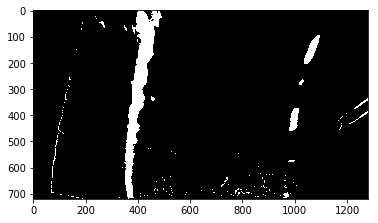
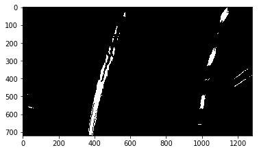
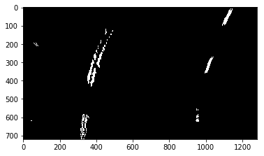
Here's my output for this step for all the test images as well as an additional test image. What I found was that these were the thresholdings which worked for most of the images.
3. Describe how (and identify where in your code) you performed a perspective transform and provide an example of a transformed image.
In the 5th code cell of my IPython notebook I used the the undistorted image and computed the perspective transform using the cv2.getPerspectiveTransform() function. I hardcoded the source (src) by defining them on the lane markings in the undistorted straight lines images and the destination (dst) points by centering around the middle of the image. The following were used:
| Source | Destination |
|---|---|
| 215, 710 | 340, 720 |
| 595, 450 | 320, 0 |
| 690, 450 | 940, 0 |
| 1100, 710 | 940, 720 |
I verified that my perspective transform was working as expected by drawing the src and dst points onto a test image and its warped counterpart to verify that the lines appear parallel in the warped image.
4. Describe how (and identify where in your code) you identified lane-line pixels and fit their positions with a polynomial.
By using a histogram of the sum of column pixel values I was able to find the starting points of the lane lines, as seen in code cell 8 of my notebook. Thereafter I used a sliding window to find the rest of the lane markings. A second order polynomial were then fitted to all the found lane marking points (one for left and another for right).
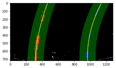
If I had already found the lane markings equations in an earlier image I used this knowledge to not need to search through the whole image again. Instead I searched close to the earlier function predictions, as seen in code cell 10 (This can be seen better in the final pipeline in cell 17 and 22). Here is an example of the output:
I used some sanity checking on my found lane marking equations to disregard unreasonable ones. Thereafter I was also averaging the new and the last lane markings. If I didn't find any lane markings I was using the equation from last found lane markings instead, thereafter I was doing a new histogram search in the next frame.
5. Describe how (and identify where in your code) you calculated the radius of curvature of the lane and the position of the vehicle with respect to center.
The vehicle position was calculated based on the offset of the lane markings to the middle of the camera image (we assume that the camera is placed in the middle of the vehicle). This can be seen in code cell 12 of my notebook.
The curvature was calculated for each lane marking (left and right) based on an equation which is explained here. This can be seen in code cell 13 of my IPython notebook.
Conversion from pixels to meters was also made for both cases, which is defined based on pixel values in the warped (transformed) image and the assumption that the lane width is 3,7m and that we are predicting 30m ahead.
6. Provide an example image of your result plotted back down onto the road such that the lane area is identified clearly.
I implemented this step in code cell 14. Here is an example of my result on a test image:
Pipeline (video)
1. Provide a link to your final video output. Your pipeline should perform reasonably well on the entire project video (wobbly lines are ok but no catastrophic failures that would cause the car to drive off the road!).
Here's a link to my video result
Discussion
1. Briefly discuss any problems / issues you faced in your implementation of this project. Where will your pipeline likely fail? What could you do to make it more robust?
Here I'll talk about the approach I took, what techniques I used, what worked and why, where the pipeline might fail and how I might improve it if I were going to pursue this project further.
I think the most important part of the project is to find a good thresholding function. I plotted some different thresholdings and tried to see which thresholdings could capture different parts of the lane markings most correctly in different images and thereafter chose to combine them to get a robust system which can detect lane markings in a lot of different environments.
I still think that my solution is likely to fail when there is big contrast differences in the images. To make it more robust I will need to analyse for example some image frames of the challenge_video as well as from the harder_challenge_video.
For the polynomial fit I disregarded fits that was a lot different compared with my last one and used an average over the last 2 frames. I think I could expand this even further. Since I made the assumption that fits that was changing a lot was not reasonalbe (i.e. I disregarded them) my approach may be too restrictive for the challenge track.
During perspective transform I made the assumption that the lane is flat, but for example in the harder_challenge video it is not, why I would like to investigate how this may affect the system. In that video we can also see that some curves are S-shaped, why a higher order polynomial may be more appropriate.
To see the drawback of my solution it is possible to watch my algorithm in action on the challenge and harder_challenge video.
