The Institute of Mixture Modeling for Equity-Oriented Researchers, Scholars, and Educators (IMMERSE) is an IES funded training grant (R305B220021) to support education scholars in integrating mixture modeling into their research.
Visit our Website to learn more about the IMMERSE project.
Follow us on Twitter for updates on posted resources!
Visit our GitHub account to follow along with this tutorial & others.
This
Rtutorial automates the 3-step ML auxiliary variable procedure using theMplusAutomationpackage (Hallquist & Wiley, 2018) to estimate models and extract relevant parameters. To learn more about auxiliary variable integration methods and why multi-step methods are necessary for producing un-biased estimates see Asparouhov & Muthén (2014).
The motivation for this tutorial is that conducting the 3-step manually is highly error prone as it requires pulling logit values estimated in the step-1 model and adding them in the model statement of the step-2 model (i.e., lots of copying & pasting). In contrast, this approach is fully replicable and provides clear documentation which translates to more reliable research. Also, it saves time!
\newpage
How to reference this tutorial:
Garber, A. C. (2021). 3-Step ML Auxiliary Variable Integration Using MplusAutomation. Retrieved from psyarxiv.com/phtxa
Follow along! Link to Github repository:
https://github.com/immerse-ucsb/3step-ML-auto
Load packages
library(MplusAutomation) # Conduit between R & Mplus
library(glue)            # Pasting R code into strings
library(here)            # Location, location, location
library(tidyverse)       # Tidyness
library(gt)              # Tables
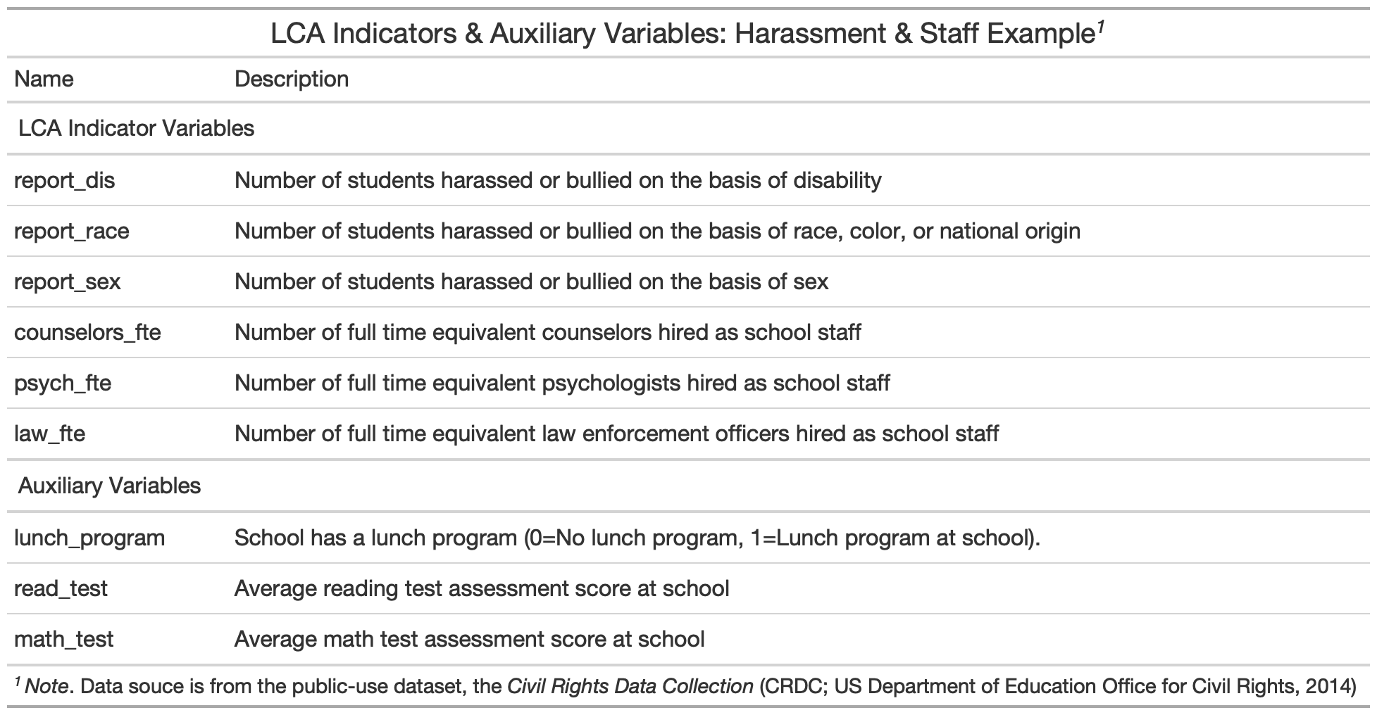
The CRDC is a federally mandated school and district level data collection effort that occurs every other year. This public data is currently available for selected variables across 4 years (2011, 2013, 2015, 2017) and all US states. In the following tutorial six focal variables are utilized as indicators of the latent class model; three variables which report on harassment/bullying in schools based on disability, race, or sex, and three variables on full-time equivalent school staff employees (counselor, psychologist, law enforcement). For this example, we utilize a sample of schools from the state of Arizona reported in 2017.
Information about CRCD: https://www2.ed.gov/about/offices/list/ocr/data.html
Data access (R): https://github.com/UrbanInstitute/education-data-package-r
Read in CSV data file from the data subfolder
data_3step <- read_csv(here("data", "crdc_aux_data.csv"))
\newpage
Step 1 - Estimate the unconditional model with all covariate & distal outcome variables mentioned in the auxiliary statement.
NOTE: In this example, Mplus input and output files are directed to the sub-folder 3step_mplus. Due to the fact that adding auxiliary variables is conducted after enumeration, generally other sub-folders will exist in the top-most Rproject folder such as enum_mplus, data, and figures.
m_step1  <- mplusObject(
  TITLE = "Step1  (MANUAL 3-STEP ML APPROACH)",
  VARIABLE =
   "categorical = report_dis report_race report_sex counselors_fte psych_fte law_fte;

    usevar = report_dis report_race report_sex counselors_fte psych_fte law_fte;

    classes = c(3);

    !!! All auxiliary variables to be considered in the final model should be listed here !!!
    auxiliary =
    lunch_program read_test math_test;",

  ANALYSIS =
   "estimator = mlr;
    type = mixture;
    starts = 500 100;

    !!! to replicate class order use, `optseed = 887580;` !!!",

  SAVEDATA =
   "!!! This saved dataset will contain class probabilities and modal assignment columns !!!
    File=3step_savedata.dat;
    Save=cprob;
    Missflag= 999;",

  PLOT =
    "type = plot3;
    series = report_dis report_race report_sex counselors_fte psych_fte law_fte(*);",

  usevariables = colnames(data_3step),
  rdata = data_3step)

m_step1_fit <- mplusModeler(m_step1,
                 dataout=here("3step_mplus", "Step1_3step.dat"),
                 modelout=here("3step_mplus", "Step1_3step.inp") ,
                 check=TRUE, run = TRUE, hashfilename = FALSE)
Extract logits for the classification probabilities for the most likely latent class
logit_cprobs <- as.data.frame(m_step1_fit[["results"]]
                                         [["class_counts"]]
                                         [["logitProbs.mostLikely"]])
Extract saved data from the step 1 model mplusObject named "m_step1_fit"
savedata <- as.data.frame(m_step1_fit[["results"]]
                                     [["savedata"]])
Rename the column in savedata for "C" and change to "N"
colnames(savedata)[colnames(savedata)=="C"] <- "N"
This model is estimated to check that the class proportions are approximately the same as in step 1.
m_step2  <- mplusObject(
  TITLE = "Step2  (MANUAL 3-STEP ML APPROACH)",

  VARIABLE =
 "nominal=N;
  USEVAR = n;
  missing are all (999);
  classes = c(3); ",

  ANALYSIS =
 "estimator = mlr;
  type = mixture;
  starts = 0;",

  MODEL =
    glue(
 "%C#1%
  [n#1@{logit_cprobs[1,1]}];
  [n#2@{logit_cprobs[1,2]}];

  %C#2%
  [n#1@{logit_cprobs[2,1]}];
  [n#2@{logit_cprobs[2,2]}];

  %C#3%
  [n#1@{logit_cprobs[3,1]}];
  [n#2@{logit_cprobs[3,2]}];"),

  usevariables = colnames(savedata),
  rdata = savedata)

m_step2_fit <- mplusModeler(m_step2,
                 dataout=here("3step_mplus", "Step2_3step.dat"),
                 modelout=here("3step_mplus", "Step2_3step.inp"),
                 check=TRUE, run = TRUE, hashfilename = FALSE)
Specification details:
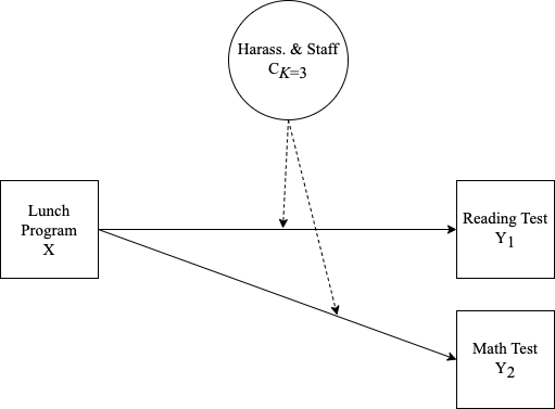
- This example contains two distal outcomes (
read_test&math_test) and one binary covariate (lunch_program). - Under each class-specific statement (e.g.,
%C#1%) the distal outcomes are mentioned to estimate the intercept parameters. - Moderation is specified by mentioning the
"outcome ON covariate;"syntax under each of the class-specific statements. - Note that the binary covariate is centered so that reported distal means (intercepts) are estimated at the weighted average of
lunch_program.
m_step3  <- mplusObject(
  TITLE = "Step3  (MANUAL 3-STEP ML APPROACH)",

  VARIABLE =
 "nominal = N;
  usevar = n;
  missing are all (999);

  usevar = lunch_pr read_tes math_tes;
  classes = c(3); ",

  DEFINE =
 "Center lunch_pr (Grandmean);",

  ANALYSIS =
 "estimator = mlr;
  type = mixture;
  starts = 0;",

  MODEL =
  glue(
 "!!! OUTCOMES = read_tes math_tes !!!
  !!! MODERATOR = lunch_pr !!!

  %OVERALL%
  read_tes on lunch_pr;
  read_tes;

  math_tes on lunch_pr;
  math_tes;

  %C#1%
  [n#1@{logit_cprobs[1,1]}];
  [n#2@{logit_cprobs[1,2]}];

  [read_tes](m01);
  read_tes;                    !!! estimate conditional intercept !!!
  read_tes on lunch_pr (s01);    !!! estimate conditional regression !!!

  [math_tes] (m1);
  math_tes;
  math_tes on lunch_pr (s1);

  %C#2%
  [n#1@{logit_cprobs[2,1]}];
  [n#2@{logit_cprobs[2,2]}];

  [read_tes](m02);
  read_tes;
  read_tes on lunch_pr (s02);

  [math_tes] (m2);
  math_tes;
  math_tes on lunch_pr (s2);

  %C#3%
  [n#1@{logit_cprobs[3,1]}];
  [n#2@{logit_cprobs[3,2]}];

  [read_tes](m03);
  read_tes;
  read_tes on lunch_pr (s03);

  [math_tes] (m3);
  math_tes;
  math_tes on lunch_pr (s3);"),

  MODELCONSTRAINT =
 "New (diff12 diff13
  diff23 slope12 slope13
  slope23 ndiff12 ndiff13
  ndiff23 nslope12 nslope13
  nslope23);

  diff12 = m1-m2;   ndiff12 = m01-m02;
  diff13 = m1-m3;   ndiff13 = m01-m03;
  diff23 = m2-m3;   ndiff23 = m02-m03;
  slope12 = s1-s2;  nslope12 = s01-s02;
  slope13 = s1-s3;  nslope13 = s01-s03;
  slope23 = s2-s3;  nslope23 = s02-s03;",

  MODELTEST =
  ## NOTE: Only a single Wald test can be conducted per model run. Therefore,
  ## this example requires running separate models for each omnibus test (e.g.,
  ## 4 models; 2 outcomes and 2 slope coefficients). This can be done by
  ## commenting out all but one test and then estimating multiple versions of the model.

 "!m01=m02;    !!! Distal outcome omnibus Wald test for `read_tes` !!!
  !m02=m03;

  !s01=s02;   !!! Slope difference omnibus Wald test for `read_tes on lunch_pr` !!!
  !s02=s03;

  m1=m2;       !!! Distal outcome omnibus Wald test for `math_tes` !!!
  m2=m3;

  !s1=s2;      !!! Slope difference omnibus Wald test `math_tes on lunch_pr` !!!
  !s2=s3;


 ",

  usevariables = colnames(savedata),
  rdata = savedata)

m_step3_fit <- mplusModeler(m_step3,
                 dataout=here("3step_mplus", "Step3_3step.dat"),
                 modelout=here("3step_mplus", "Step3_3step.inp"),
                 check=TRUE, run = TRUE, hashfilename = FALSE)
End of 3-Step Procedure
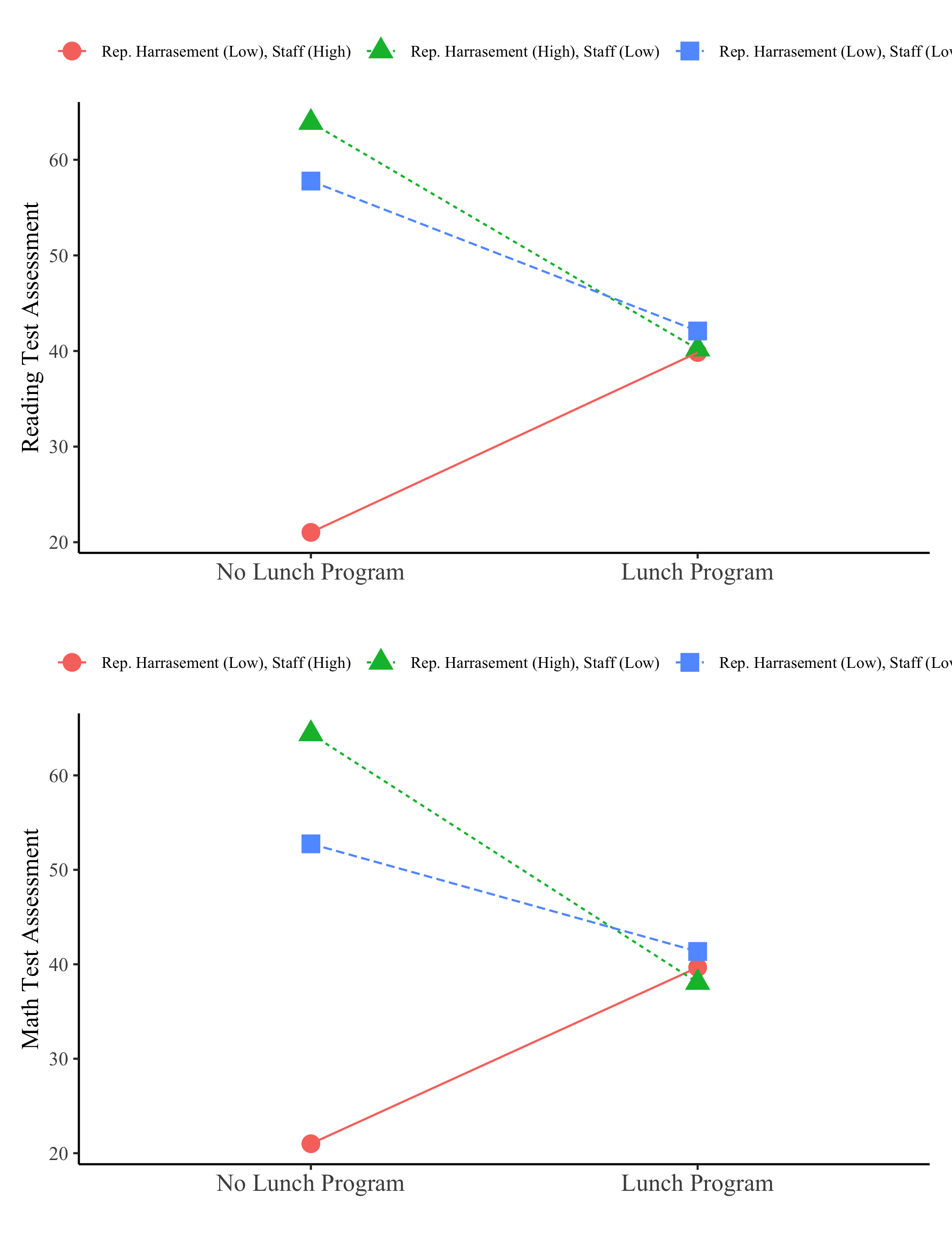
NOTE: The next video in this series will include a detailed tutorial on how to interpret auxiliary variable output (i.e. distal outcomes & covariates) in the context of moderation. This tutorial will also cover
Rcode to generate figures for visualizing the results.
Asparouhov, T., & Muthén, B. O. (2014). Auxiliary variables in mixture modeling: Three-step approaches using Mplus. Structural Equation Modeling, 21, 329–341. http://dx.doi.org/10.1080/10705511.2014.915181
Hallquist, M. N., & Wiley, J. F. (2018). MplusAutomation: An R Package for Facilitating Large-Scale Latent Variable Analyses in Mplus. Structural equation modeling: a multidisciplinary journal, 25(4), 621-638.
Müller, Kirill. (2017). Here: A Simpler Way to Find Your Files. https://CRAN.R-project.org/package=here.
Muthén, B. O., Muthén, L. K., & Asparouhov, T. (2017). Regression and mediation analysis using Mplus. Los Angeles, CA: Muthén & Muthén.
Muthén, L.K. and Muthén, B.O. (1998-2017). Mplus User's Guide. Eighth Edition. Los Angeles, CA: Muthén & Muthén
US Department of Education Office for Civil Rights. (2014). Civil rights data collection data snapshot: School discipline. Issue brief no. 1.
R Core Team (2017). R: A language and environment for statistical computing. R Foundation for Statistical Computing, Vienna, Austria. URL http://www.R-project.org/
Wickham et al., (2019). Welcome to the tidyverse. Journal of Open Source Software, 4(43), 1686, https://doi.org/10.21105/joss.01686


