The Institute of Mixture Modeling for Equity-Oriented Researchers, Scholars, and Educators (IMMERSE) is an IES funded training grant (R305B220021) to support education scholars in integrating mixture modeling into their research.
Visit our Website to learn more about the IMMERSE project.
Follow us on Twitter for updates on posted resources!
Visit our GitHub account to follow along with this tutorial & others.
This tutorial covers the interpretation of the results of a mixture model with auxiliary variables. Specifically, an LCA model is specified with relations to covariate and distal outcomes in three examples. Auxiliary variable integration is specified using the 3-step ML auxiliary variable procedure using the
MplusAutomationpackage (Hallquist & Wiley, 2018; Vermunt, 2010; Asparouhov & Muthén, 2014). In addition to running the models this tutorial covers plotting the results of distal outcome means and covariate relations in the context of moderation (see example; Nylund-Gibson et al., 2022).
Follow along! Link to Github repository:
https://github.com/immerse-ucsb/interpret-aux-vars
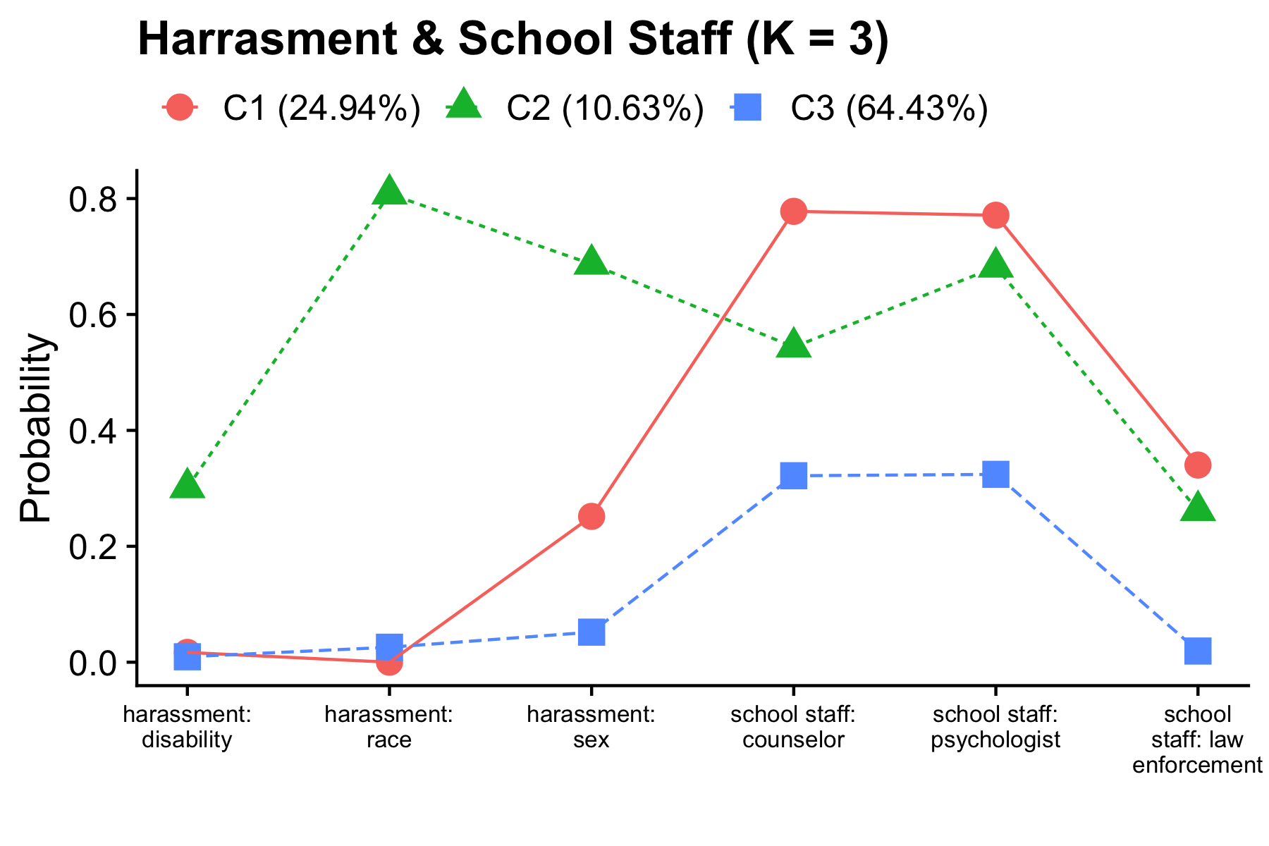
The CRDC is a federally mandated school and district level data collection effort that occurs every other year. This public data is currently available for selected variables across 4 years (2011, 2013, 2015, 2017) and all US states. In the following tutorial six focal variables are utilized as indicators of the latent class model; three variables which report on harassment/bullying in schools based on disability, race, or sex, and three variables on full-time equivalent school staff employees (counselor, psychologist, law enforcement). For this example, we utilize a sample of schools from the state of Arizona reported in 2017.
Information about CRCD: https://www2.ed.gov/about/offices/list/ocr/data.html
Data access (R): https://github.com/UrbanInstitute/education-data-package-r
LCA Enumeration: https://github.com/immerse-ucsb/lca_enum
3-Step Method: https://github.com/immerse-ucsb/3-Step-ML-auto
Getting started: Load packages & Read in CSV data file from the data subfolder
library(MplusAutomation) # Conduit between R & Mplus
library(glue)            # Pasting R code into strings
library(here)            # Location, location, location
library(tidyverse)       # Tidyness
library(gt)              # Tables
library(cowplot)         # ggplot theme
library(reshape2)        # melt() function
data_3step <- read_csv(here("data", "crdc_aux_data.csv"))
Note: Model steps in this tutorial are labeled differently than in the technical documentation for the 3-step procedure (i.e., Vermunt, 2010; Asparouhov & Muthén, 2014).
m_step1  <- mplusObject(
  TITLE = "Step1  (MANUAL 3-STEP ML APPROACH)",
  VARIABLE =
   "categorical = report_dis report_race report_sex counselors_fte psych_fte law_fte;

    usevar = report_dis report_race report_sex counselors_fte psych_fte law_fte;

    classes = c(3);

    !!! All auxiliary variables to be considered in the final model should be listed here !!!
    auxiliary =
    lunch_program title1_e title1_s read_test math_test;",

  ANALYSIS =
   "estimator = mlr;
    type = mixture;
    starts = 500 100;

    !!! to replicate class order use, `optseed = 887580;` !!!",

  SAVEDATA =
   "!!! This saved dataset will contain class probabilities and modal assignment columns !!!
    File=3step_savedata.dat;
    Save=cprob;
    Missflag= 999;",

  PLOT =
    "type = plot3;
    series = report_dis report_race report_sex counselors_fte psych_fte law_fte(*);",

  usevariables = colnames(data_3step),
  rdata = data_3step)

m_step1_fit <- mplusModeler(m_step1,
                 dataout=here("3step_mplus", "Step1_3step.dat"),
                 modelout=here("3step_mplus", "Step1_3step.inp") ,
                 check=TRUE, run = TRUE, hashfilename = FALSE)

- - -
# Step 2 - Extract logits & saved data from the step 1 unconditional model.
- - -

logit_cprobs <- as.data.frame(m_step1_fit[["results"]]
                                         [["class_counts"]]
                                         [["logitProbs.mostLikely"]])

savedata <- as.data.frame(m_step1_fit[["results"]]
                                     [["savedata"]])

colnames(savedata)[colnames(savedata)=="C"] <- "N"

- - -
# Step 2 (part 2) - Estimate the unconditional model with logits from step 2.
- - -

m_step2  <- mplusObject(
  TITLE = "Step2  (MANUAL 3-STEP ML APPROACH)",

  VARIABLE =
 "nominal=N;
  USEVAR = n;
  missing are all (999);
  classes = c(3); ",

  ANALYSIS =
 "estimator = mlr;
  type = mixture;
  starts = 0;",

  MODEL =
    glue(
 "%C#1%
  [n#1@{logit_cprobs[1,1]}];
  [n#2@{logit_cprobs[1,2]}];

  %C#2%
  [n#1@{logit_cprobs[2,1]}];
  [n#2@{logit_cprobs[2,2]}];

  %C#3%
  [n#1@{logit_cprobs[3,1]}];
  [n#2@{logit_cprobs[3,2]}];"),

  usevariables = colnames(savedata),
  rdata = savedata)

m_step2_fit <- mplusModeler(m_step2,
                 dataout=here("3step_mplus", "Step2_3step.dat"),
                 modelout=here("3step_mplus", "Step2_3step.inp"),
                 check=TRUE, run = TRUE, hashfilename = FALSE)
Specify the distal outcome model
m_step3  <- mplusObject(
  TITLE = "Distal Outcome Model (Step3)",

  VARIABLE =
 "nominal = N;
  usevar = n;
  missing are all (999);

  usevar = read_tes math_tes;
  classes = c(3); ",

  ANALYSIS =
 "estimator = mlr;
  type = mixture;
  starts = 0;",

  MODEL =
  glue(
 "!!! DISTAL OUTCOMES = read_tes math_tes !!!

  %OVERALL%

  read_tes;
  math_tes;

  %C#1%
  [n#1@{logit_cprobs[1,1]}];
  [n#2@{logit_cprobs[1,2]}];

  [read_tes](m01);               !!! estimate conditional intercept mean !!!
  read_tes;                      !!! estimate conditional intercept variance !!!

  [math_tes] (m1);
  math_tes;

  %C#2%
  [n#1@{logit_cprobs[2,1]}];
  [n#2@{logit_cprobs[2,2]}];

  [read_tes](m02);
  read_tes;

  [math_tes] (m2);
  math_tes;

  %C#3%
  [n#1@{logit_cprobs[3,1]}];
  [n#2@{logit_cprobs[3,2]}];

  [read_tes](m03);
  read_tes;

  [math_tes] (m3);
  math_tes;  "),

  MODELCONSTRAINT =
 "New (rdiff12 rdiff13
  rdiff23 mdiff12 mdiff13
  mdiff23);

  rdiff12 = m1-m2;   mdiff12 = m01-m02;
  rdiff13 = m1-m3;   mdiff13 = m01-m03;
  rdiff23 = m2-m3;   mdiff23 = m02-m03;",

  MODELTEST =
  ## NOTE: Only a single Wald test can be conducted per model run. Therefore,
  ## this example requires running separate models for each omnibus test (e.g.,
  ## 2 models for each outcome variable). This can be done by commenting out
  ## all but one test and then estimating multiple versions of the model.

 "m01=m02;    !!! Distal outcome omnibus Wald test for `read_tes` !!!
  m02=m03;

  !m1=m2;       !!! Distal outcome omnibus Wald test for `math_tes` !!!
  !m2=m3; ",

  usevariables = colnames(savedata),
  rdata = savedata)

m_step3_fit <- mplusModeler(m_step3,
                 dataout=here("3step_mplus", "EX1_Distal_Model.dat"),
                 modelout=here("3step_mplus", "EX1_Distal_Model.inp"),
                 check=TRUE, run = TRUE, hashfilename = FALSE)
This syntax reads in the Step3 model & extract model parameter estimates.
model_step3 <- readModels(here("3step_mplus", "EX1_Distal_Model.out"), quiet = TRUE)

model_step3 <- data.frame(model_step3$parameters$unstandardized)
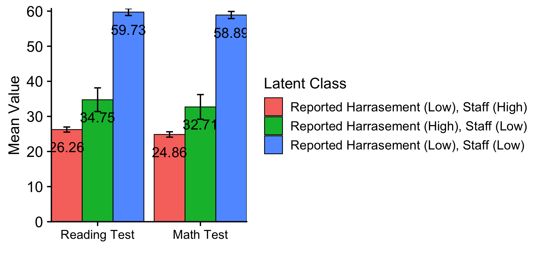
This syntax is used to create the data-frame that produces the distal outcome bar plot.
distal_data <- model_step3 %>%
  filter(paramHeader == "Means") %>%
  filter(param == c("READ_TES","MATH_TES")) %>%
  mutate(param = case_when(
      param == "READ_TES" ~ "Reading Test",
      param == "MATH_TES" ~ "Math Test")) %>%
  mutate(LatentClass = factor(LatentClass,
      labels = c("Reported Harrasement (Low), Staff (High)",
                 "Reported Harrasement (High), Staff (Low)",
                 "Reported Harrasement (Low), Staff (Low)"))) %>%
  mutate(value_labels = round(est,2))
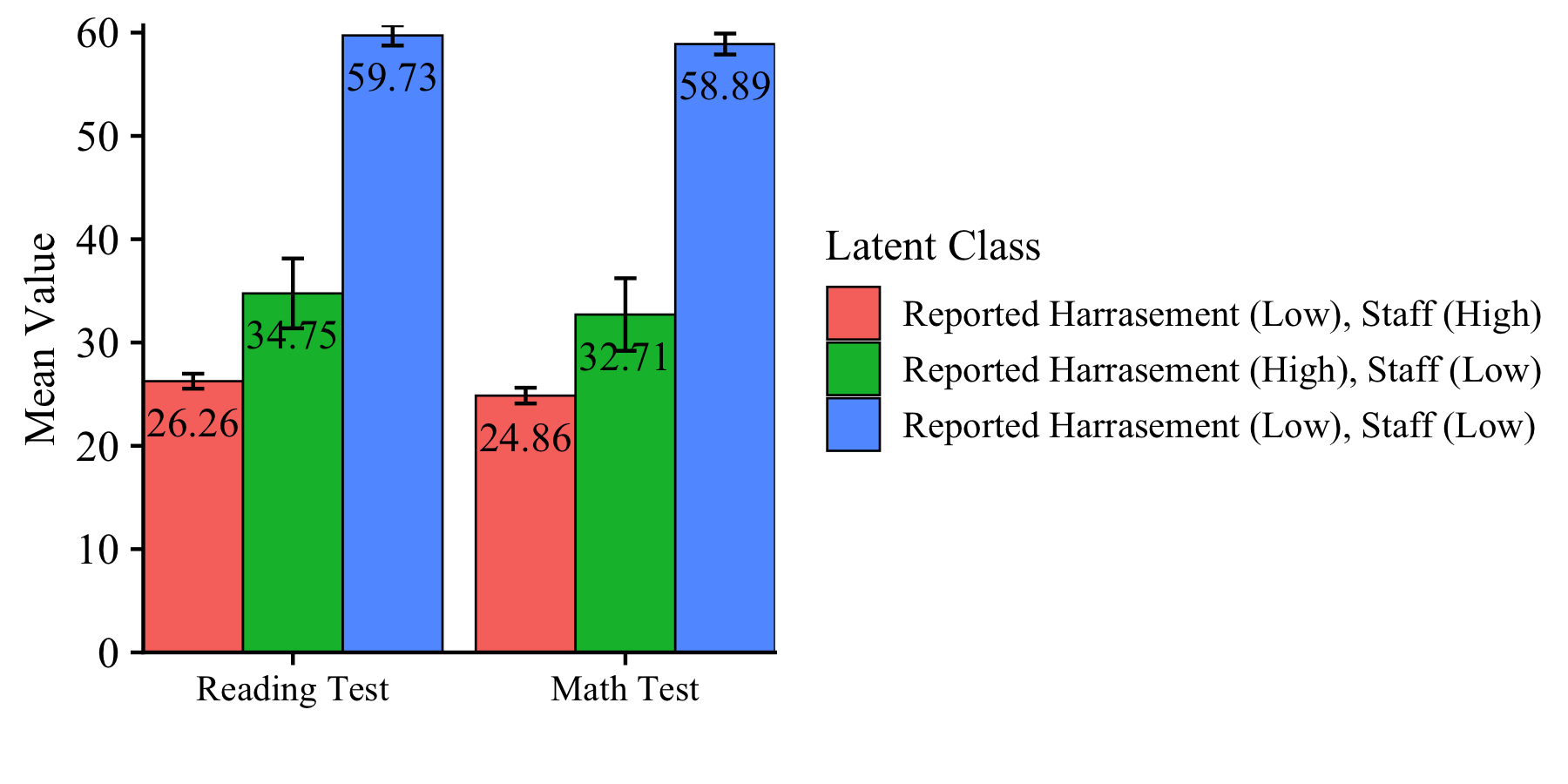
Plot distal outcomes grouped by class
ggplot(distal_data,
       aes(fill=LatentClass, y=est, x=fct_rev(param))) +
  geom_bar(position="dodge", stat="identity", color="black", size=.3) +
  geom_errorbar( aes(ymin=est-se, ymax=est+se),
                 width=.2, position=position_dodge(.9)) +
  geom_text(aes(y = est -5, label = value_labels),
            size=4, position=position_dodge(.9)) +
  theme_cowplot() +
  labs(x = "", y = "Mean Value", fill = "Latent Class") +
  theme(text=element_text(size=12),
        axis.text.x=element_text(size=10)) +
        coord_cartesian(expand = FALSE)
ggsave(here("figures","EX1_Distal_barplot.png"), dpi=300, height=3, width=6, units="in")
Specification details:
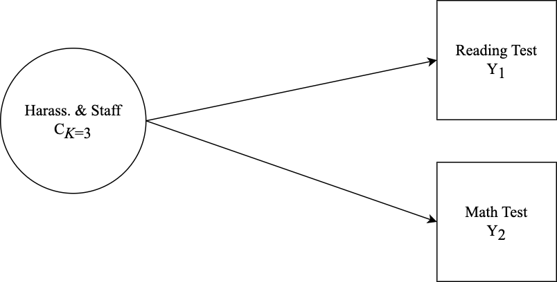
- This example contains two distal outcomes (
read_test&math_test) and one binary covariate (lunch_program). - Under each class-specific statement (e.g.,
%C#1%) the distal outcome means & variances are mentioned to allow these parameters to vary by class. - Note that the binary covariate is centered so that reported distal means (intercepts) are estimated at the average of
lunch_program.
m_step3  <- mplusObject(
  TITLE = "Distal Outcome Model with Control Covariate (Step3)",

  VARIABLE =
 "nominal = N;
  usevar = n;
  missing are all (999);

  usevar = lunch_pr read_tes math_tes;
  classes = c(3); ",

  DEFINE =
 "Center lunch_pr (Grandmean);",

  ANALYSIS =
 "estimator = mlr;
  type = mixture;
  starts = 0;",

  MODEL =
  glue(
 "!!! DISTAL OUTCOMES = read_tes math_tes !!!
  !!! COVARIATE = lunch_pr !!!

  %OVERALL%
  c on lunch_pr;                 !!! estimate covariate as predictor of latent class !!!

  read_tes on lunch_pr;          !!! estimate the direct effect of Y on X !!!
  math_tes on lunch_pr;

  read_tes;
  math_tes;

  %C#1%
  [n#1@{logit_cprobs[1,1]}];
  [n#2@{logit_cprobs[1,2]}];

  [read_tes](m01);               !!! estimate conditional intercept mean !!!
  read_tes;                      !!! estimate conditional intercept variance !!!

  [math_tes] (m1);
  math_tes;

  %C#2%
  [n#1@{logit_cprobs[2,1]}];
  [n#2@{logit_cprobs[2,2]}];

  [read_tes](m02);
  read_tes;

  [math_tes] (m2);
  math_tes;

  %C#3%
  [n#1@{logit_cprobs[3,1]}];
  [n#2@{logit_cprobs[3,2]}];

  [read_tes](m03);
  read_tes;

  [math_tes] (m3);
  math_tes;  "),

  MODELCONSTRAINT =
 "New (rdiff12 rdiff13
  rdiff23 mdiff12 mdiff13
  mdiff23);

  rdiff12 = m1-m2;   mdiff12 = m01-m02;
  rdiff13 = m1-m3;   mdiff13 = m01-m03;
  rdiff23 = m2-m3;   mdiff23 = m02-m03;",

  MODELTEST =
  ## NOTE: Only a single Wald test can be conducted per model run. Therefore,
  ## this example requires running separate models for each omnibus test (e.g.,
  ## 2 models for each outcome variable). This can be done by commenting out
  ## all but one test and then estimating multiple versions of the model.

 "!m01=m02;    !!! Distal outcome omnibus Wald test for `read_tes` !!!
  !m02=m03;

  m1=m2;       !!! Distal outcome omnibus Wald test for `math_tes` !!!
  m2=m3;

 ",

  usevariables = colnames(savedata),
  rdata = savedata)

m_step3_fit <- mplusModeler(m_step3,
                 dataout=here("3step_mplus", "EX2_Dist_Cov_Model.dat"),
                 modelout=here("3step_mplus", "EX2_Dist_Cov_Model.inp"),
                 check=TRUE, run = TRUE, hashfilename = FALSE)
Note: The distal outcome means are estimated at the average of the covariate (lunch_pr). This is specified by centering lunch program as shown in the Step-3 model syntax.
This syntax reads in the data, extracts relevant parameters, and generates the plot.
model_step3 <- readModels(here("3step_mplus", "EX2_Dist_Cov_Model.out"), quiet = TRUE)

model_step3 <- data.frame(model_step3$parameters$unstandardized)

distal_data <- model_step3 %>%
  filter(paramHeader == "Intercepts") %>%
  filter(param == c("READ_TES","MATH_TES")) %>%
  mutate(param = case_when(
      param == "READ_TES" ~ "Reading Test",
      param == "MATH_TES" ~ "Math Test")) %>%
  mutate(LatentClass = factor(LatentClass,
      labels = c("Reported Harrasement (Low), Staff (High)",
                 "Reported Harrasement (High), Staff (Low)",
                 "Reported Harrasement (Low), Staff (Low)"))) %>%
  mutate(value_labels = round(est,2))

ggplot(distal_data,
       aes(fill=LatentClass, y=est, x=fct_rev(param))) +
  geom_bar(position="dodge", stat="identity", color="black", size=.3) +
  geom_errorbar( aes(ymin=est-se, ymax=est+se),
                 width=.2, position=position_dodge(.9)) +
  geom_text(aes(y = est -4, label = value_labels),
            size=4, position=position_dodge(.9)) +
  theme_cowplot() +
  labs(x = "", y = "Mean Value", fill = "Latent Class") +
  theme(text=element_text(size=12),
        axis.text.x=element_text(size=10)) +
        coord_cartesian(expand = FALSE)
ggsave(here("figures","EX2_Distal_barplot.png"), dpi=300, height=3, width=6, units="in")
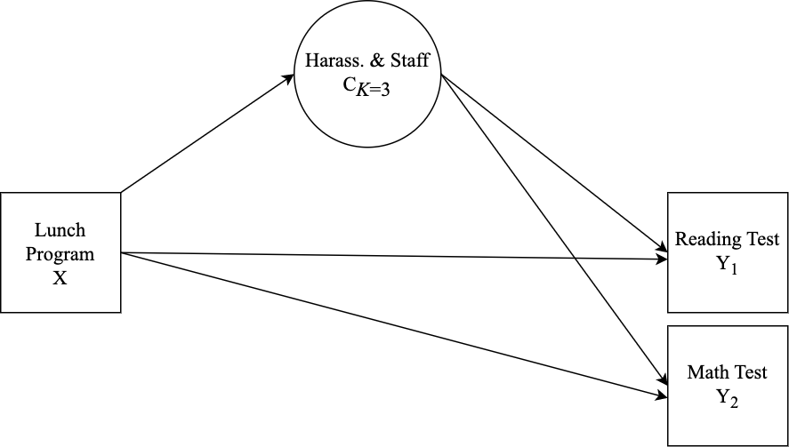
Specification details:
- This example contains two distal outcomes (
read_test&math_test) and one binary covariate (lunch_program). - Under each class-specific statement (e.g.,
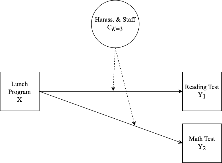
%C#1%) the distal outcome means & variances are mentioned to allow these parameters to vary by class. - Moderation is specified by mentioning the
"outcome ON covariate;"syntax under each of the class-specific statements. - Note that the binary covariate is centered so that reported distal means (intercepts) are estimated at the average of
lunch_program.
m_step3  <- mplusObject(
  TITLE = "Step3  (MANUAL 3-STEP ML APPROACH)",

  VARIABLE =
 "nominal = N;
  usevar = n;
  missing are all (999);

  usevar = lunch_pr read_tes math_tes;
  classes = c(3); ",

  DEFINE =
 "Center lunch_pr (Grandmean);",

  ANALYSIS =
 "estimator = mlr;
  type = mixture;
  starts = 0;",

  MODEL =
  glue(
 "!!! OUTCOMES = read_tes math_tes !!!
  !!! COVARIATE = lunch_pr !!!
  !!! MODERATOR = C !!!

  %OVERALL%
  read_tes on lunch_pr;
  read_tes;

  math_tes on lunch_pr;
  math_tes;

  %C#1%
  [n#1@{logit_cprobs[1,1]}];
  [n#2@{logit_cprobs[1,2]}];

  [read_tes](m01);
  read_tes;                    !!! estimate conditional intercept !!!
  read_tes on lunch_pr (s01);    !!! estimate conditional regression !!!

  [math_tes] (m1);
  math_tes;
  math_tes on lunch_pr (s1);

  %C#2%
  [n#1@{logit_cprobs[2,1]}];
  [n#2@{logit_cprobs[2,2]}];

  [read_tes](m02);
  read_tes;
  read_tes on lunch_pr (s02);

  [math_tes] (m2);
  math_tes;
  math_tes on lunch_pr (s2);

  %C#3%
  [n#1@{logit_cprobs[3,1]}];
  [n#2@{logit_cprobs[3,2]}];

  [read_tes](m03);
  read_tes;
  read_tes on lunch_pr (s03);

  [math_tes] (m3);
  math_tes;
  math_tes on lunch_pr (s3);"),

  MODELCONSTRAINT =
 "New (rdiff12 rdiff13
  rdiff23 rslope12 rslope13
  rslope23 mdiff12 mdiff13
  mdiff23 mslope12 mslope13
  mslope23);

  rdiff12 = m1-m2;   mdiff12 = m01-m02;
  rdiff13 = m1-m3;   mdiff13 = m01-m03;
  rdiff23 = m2-m3;   mdiff23 = m02-m03;
  rslope12 = s1-s2;  mslope12 = s01-s02;
  rslope13 = s1-s3;  mslope13 = s01-s03;
  rslope23 = s2-s3;  mslope23 = s02-s03;",

  MODELTEST =
  ## NOTE: Only a single Wald test can be conducted per model run. Therefore,
  ## this example requires running separate models for each omnibus test (e.g.,
  ## 4 models; 2 outcomes and 2 slope coefficients). This can be done by
  ## commenting out all but one test and then estimating multiple versions of the model.

 "!m01=m02;    !!! Distal outcome omnibus Wald test for `read_tes` !!!
  !m02=m03;

  !s01=s02;   !!! Slope difference omnibus Wald test for `read_tes on lunch_pr` !!!
  !s02=s03;

  m1=m2;       !!! Distal outcome omnibus Wald test for `math_tes` !!!
  m2=m3;

  !s1=s2;      !!! Slope difference omnibus Wald test `math_tes on lunch_pr` !!!
  !s2=s3; ",

  usevariables = colnames(savedata),
  rdata = savedata)

m_step3_fit <- mplusModeler(m_step3,
                 dataout=here("3step_mplus", "EX3_Moderation_Model.dat"),
                 modelout=here("3step_mplus", "EX3_Moderation_Model.inp"),
                 check=TRUE, run = TRUE, hashfilename = FALSE)
- Intercepts are estimated at the reference level of the covariate (i.e.,
lunch_pr = 0)
Note: Here the update() function is used to take the previous model and remove the Mplus syntax within the DEFINE statement that was used to center the covariate Lunch Program. Next, the updated model input syntax is used to estimate a new model. To learn more about the update function see the MplusAutomation tutorial article (https://www.tandfonline.com/doi/pdf/10.1080/10705511.2017.1402334).
m_uncen <- update(m_step3,
  DEFINE = ~" ") # This update removes the centering syntax from the model object `m_step3`

m_uncen_fit <- mplusModeler(m_uncen,
                            dataout=here("3step_mplus", "EX3_Uncentered.dat"),
                            modelout=here("3step_mplus", "EX3_Uncentered.inp"),
                            check=TRUE, run = TRUE, hashfilename = FALSE)
This syntax reads in the Step3 model & extract model parameter estimates.
model_step3 <- readModels(here("3step_mplus", "EX3_Moderation_Model.out"), quiet = TRUE)

model_step3 <- data.frame(model_step3$parameters$unstandardized)

distal_data <- model_step3 %>%
  filter(paramHeader == "Intercepts") %>%
  mutate(param = case_when(
      param == "READ_TES" ~ "Reading Test",
      param == "MATH_TES" ~ "Math Test")) %>%
  mutate(LatentClass = factor(LatentClass,
      labels = c("Reported Harrasement (Low), Staff (High)",
                 "Reported Harrasement (High), Staff (Low)",
                 "Reported Harrasement (Low), Staff (Low)"))) %>%
  mutate(value_labels = c("36.4a", "36.3a", "44.5b", "42.8b", "44.9b", "43.4b"))

ggplot(distal_data,
       aes(fill=LatentClass, y=est, x=fct_rev(param))) +
  geom_bar(position="dodge", stat="identity", color="black", size=.3) +
  geom_errorbar( aes(ymin=est-se, ymax=est+se),
                 width=.2, position=position_dodge(.9)) +
  geom_text(aes(y = est -4, label = value_labels),
            size=4, position=position_dodge(.9)) +
  #scale_fill_grey(start = 0.6, end = 1.0) +
  theme_cowplot() +
  labs(x = "", y = "Mean Value", fill = "Latent Class") +
  theme(text=element_text(size=12),
        axis.text.x=element_text(size=10)) +
        coord_cartesian(expand = FALSE)
ggsave(here("figures","EX3_Distal_barplot.png"), dpi=300, height=3, width=6, units="in")
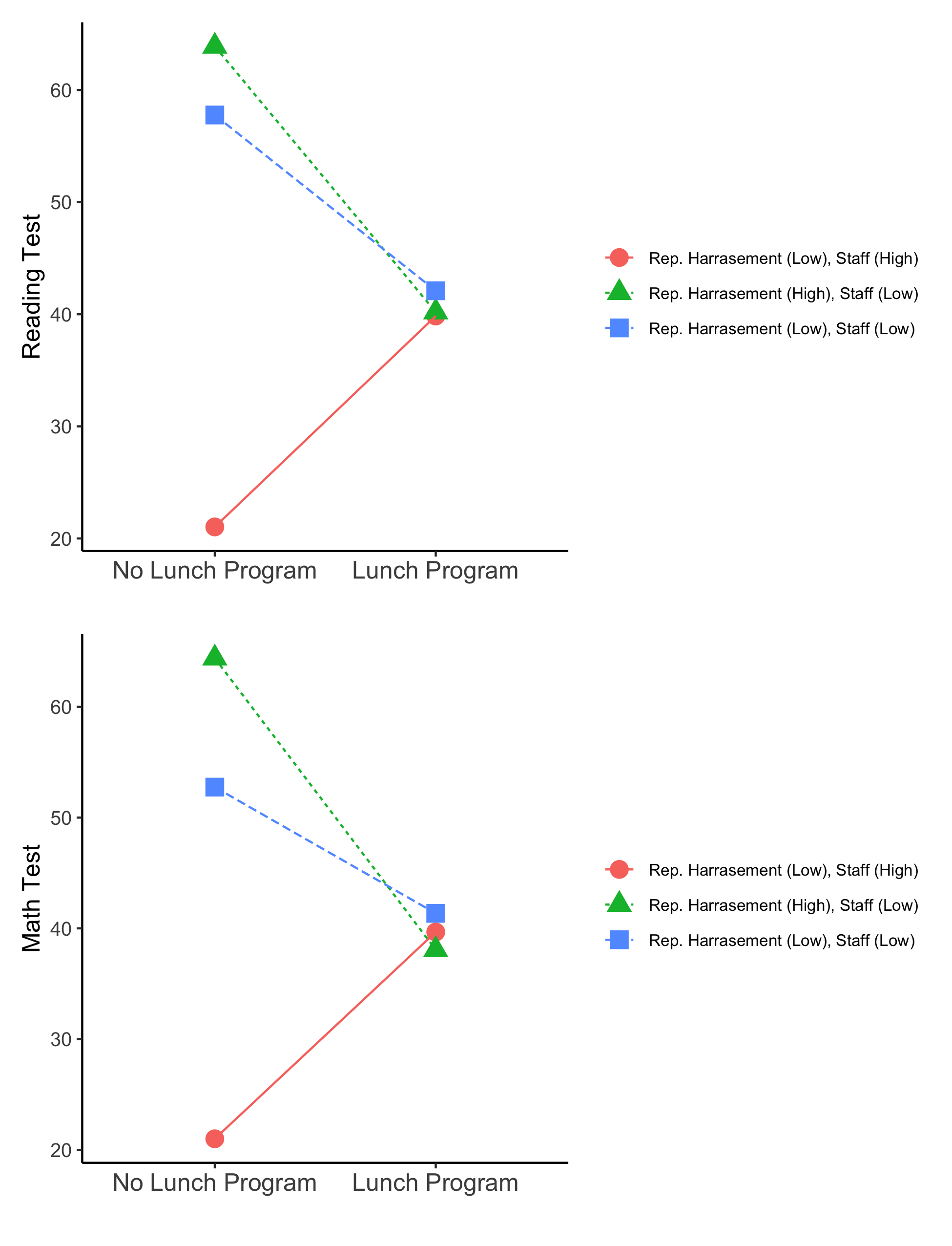
Note: The un-centered distal intercepts represent the conditional means when the binary covariate is at its first level lunch_pr = 0 (i.e., school does not have a lunch program). Therefore, the conditional mean for lunch_pr = 1 (i.e., school has lunch program) can be calculated by adding the associated slope coefficient to the intercept.
Read in the un-centered model & extract relevant parameters
model_uncen <- readModels(here("3step_mplus", "EX3_Uncentered.out"), quiet = TRUE)

model_uncen <- data.frame(model_uncen$parameters$unstandardized)

slope_data <- model_uncen %>%
  filter(str_detect(paramHeader, 'ON|Inter'))%>%
  unite("param", paramHeader:param, remove = TRUE) %>%
  mutate(param = str_replace(param, "TES.ON_LUNCH_PR", "COEF")) %>%
  mutate(param = str_remove_all(param, "Intercepts_|_TES")) %>%
  mutate(LatentClass = factor(LatentClass,
    labels = c("Rep. Harrasement (Low), Staff (High)",
               "Rep. Harrasement (High), Staff (Low)",
               "Rep. Harrasement (Low), Staff (Low)")))
Prepare reading test simple slope data
read_data <- slope_data %>%
  filter(str_detect(param, 'READ'))

read_wide <- read_data %>%
  select(param,est, LatentClass) %>%
  pivot_wider(names_from = param, values_from = est) %>%
  rename("No.Lunch.Program" = 'READ') %>%
  mutate(Lunch.Program = No.Lunch.Program + READ_COEF) %>% # calc. condit. means `LUNCH_PR = 1`
  select(-READ_COEF)

read_pos <- melt(read_wide, id.vars = "LatentClass") %>%
  mutate(variable = factor(variable,
                      levels = c("No.Lunch.Program","Lunch.Program"),
                      labels = c("No Lunch Program","Lunch Program")))
Plot reading test simple slopes
r_plot <- ggplot(read_pos,
            aes(y=value, x=variable,
                color=LatentClass,
                group=LatentClass,
                shape=LatentClass,
                lty=LatentClass)) +
  geom_point(size = 4) + geom_line() +
  xlab("") + ylab("Reading Test")  +
  theme_classic() +
  theme(text=element_text(size=12),
        axis.text.x=element_text(size=12),
        legend.text = element_text(size=8),
        legend.position = "right", legend.title = element_blank())
Prepare math test simple slope data
math_data <- slope_data %>%
  filter(str_detect(param, 'MATH'))

math_wide <- math_data %>%
  select(param,est, LatentClass) %>%
  pivot_wider(names_from = param, values_from = est) %>%
  rename("No.Lunch.Program" = 'MATH') %>%
  mutate(Lunch.Program = No.Lunch.Program + MATH_COEF) %>%   # calculate means for `Lunch.Program = 1`
  select(-MATH_COEF)

plot_math <- melt(math_wide, id.vars = "LatentClass") %>%
  mutate(variable = factor(variable,
                      levels = c("No.Lunch.Program","Lunch.Program"),
                      labels = c("No Lunch Program","Lunch Program")))
Plot math test simple slopes
m_plot <- ggplot(plot_math,
            aes(y=value, x=variable,
            color=LatentClass,
            group=LatentClass,
            shape=LatentClass,
            lty=LatentClass)) +
  geom_point(size=4) + geom_line() +
  xlab("") + ylab("Math Test") +
  theme_classic() +
  theme(text=element_text(color = "black", size=12),
        axis.text.x=element_text(size=12),
        legend.text = element_text(size=8),
        legend.position = "right", legend.title = element_blank())
library(patchwork)

r_plot / m_plot # combines plots using the {patchwork} package
ggsave(here("figures", "EX3_Simple_slopes.png"), dpi=300, height=8.5, width=6.5, units="in")
Asparouhov, T., & Muthén, B. O. (2014). Auxiliary variables in mixture modeling: Three-step approaches using Mplus. Structural Equation Modeling, 21, 329–341. http://dx.doi.org/10.1080/10705511.2014.915181
Hallquist, M. N., & Wiley, J. F. (2018). MplusAutomation: An R Package for Facilitating Large-Scale Latent Variable Analyses in Mplus. Structural equation modeling: a multidisciplinary journal, 25(4), 621-638.
Müller, Kirill. (2017). Here: A Simpler Way to Find Your Files. https://CRAN.R-project.org/package=here.
Muthén, B. O., Muthén, L. K., & Asparouhov, T. (2017). Regression and mediation analysis using Mplus. Los Angeles, CA: Muthén & Muthén.
Muthén, L.K. and Muthén, B.O. (1998-2017). Mplus User's Guide. Eighth Edition. Los Angeles, CA: Muthén & Muthén
Nylund-Gibson, K., Garber, A. C., Singh, J., Witkow, M. R., Nishina, A., & Bellmore, A. (2023). The utility of latent class analysis to understand heterogeneity in youth coping strategies: A methodological introduction. Behavioral Disorders, 48(2), 106-120.
R Core Team (2017). R: A language and environment for statistical computing. R Foundation for Statistical Computing, Vienna, Austria. URL http://www.R-project.org/
Vermunt, J. K. (2010). Latent class modeling with covariates: Two improved three-step approaches. Political Analysis, 450–469. https://doi.org/10.1093/pan/mpq025
US Department of Education Office for Civil Rights. (2014). Civil rights data collection data snapshot: School discipline. Issue brief no. 1.
Wickham et al., (2019). Welcome to the tidyverse. Journal of Open Source Software, 4(43), 1686, https://doi.org/10.21105/joss.01686


