summarytools

The following vignettes complement this page:

Recommendations for Using summarytools With Rmarkdown
Introduction to summarytools – Contents similar to this page (minus installation instructions), with fancier table stylings.

What is summarytools?

summarytools is an R package providing tools to neatly and quickly summarize data. It can also make R a little easier to learn and to use, especially for data cleaning and preliminary analysis. Four functions are at the core of the package:

freq() : frequency tables with proportions, cumulative proportions and missing data information
ctable() : cross-tabulations between two factors or any discrete data, with total, rows or columns proportions, as well as marginal totals
descr() : descriptive (univariate) statistics for numerical data
dfSummary() : Extensive data frame summaries that facilitate data cleaning and firsthand evaluation

An emphasis has been put on both what and how results are presented, so that the package can serve both as an exploration and reporting tool, used on its own for minimal reports, or with other sets of tools such as rmarkdown, and knitr.

Building on the strengths of pander and htmltools, the outputs produced by summarytools can be:

Displayed in plain text in the R console (default behaviour)
Used in Rmarkdown documents and knitted along with other text and R output
Written to html files that fire up in RStudio’s Viewer pane or in the default browser
Written to plain or Rmarkdown text files

It is also possible to include summarytools’ functions in Shiny apps.

Latest Improvements

Version 0.9 brought many changes and improvements. A summary of those changes can be found near the end of this page. Changes specific to the latest release can be found in the NEWS file.

How to install

From GitHub

This is the recommended method, as some minor fixes are made available between CRAN releases.

Magick++ Dependency on Linux and Mac OS

Before proceeding, you must install Magick++

 - deb: 'libmagick++-dev' (Debian, Ubuntu)
 - rpm: 'ImageMagick-c++-devel' (Fedora, CentOS, RHEL)
 - csw: 'imagemagick_dev' (Solaris)

On MacOS it is recommended to use install ImageMagick-6 from homebrew
with extra support for fontconfig and rsvg rendering:
   brew reinstall imagemagick@6 --with-fontconfig --with-librsvg

For older Ubuntu versions Trusty (14.04) and Xenial (16.04) use the PPA:
   sudo add-apt-repository -y ppa:opencpu/imagemagick
   sudo apt-get update
   sudo apt-get install -y libmagick++-dev

After this is done, proceed with the installation:

install.packages("devtools")
library(devtools)
install_github("rapporter/pander") # Necessary for optimal results!
install_github("dcomtois/summarytools")

From CRAN

Simply install it with install.packages():

install.packages("summarytools")

The official documentation can be found here.

The Four Core Functions

1 - freq() : Frequency Tables

The freq() function generates a table of frequencies with counts and proportions. Since GitHub uses markdown rendering, we’ve set the style argument to “rmarkdown”. When creating Rmd documents, knitr takes care of converting the generated markup characters into actual html.

library(summarytools)
freq(iris$Species, style = "rmarkdown")

Frequencies

iris$Species
Type: Factor

	Freq	% Valid	% Valid Cum.	% Total	% Total Cum.
setosa	50	33.33	33.33	33.33	33.33
versicolor	50	33.33	66.67	33.33	66.67
virginica	50	33.33	100.00	33.33	100.00
<NA>	0			0.00	100.00
Total	150	100.00	100.00	100.00	100.00

If we do not worry about missing data, we can set report.nas = FALSE:

freq(iris$Species, report.nas = FALSE, style = "rmarkdown", headings = FALSE)

	Freq	%	% Cum.
setosa	50	33.33	33.33
versicolor	50	33.33	66.67
virginica	50	33.33	100.00
Total	150	100.00	100.00

We can simplify the results further and omit the Totals row by specifying totals = FALSE, as well as omit the cumulative rows by setting cumul = FALSE.

freq(iris$Species, report.nas = FALSE, totals = FALSE, cumul = FALSE, style = "rmarkdown", headings = FALSE)

	Freq	%
setosa	50	33.33
versicolor	50	33.33
virginica	50	33.33

To get familiar with the various output styles, try different values for style – “simple”, “rmarkdown” or “grid”, and see how this affects the results in the console.

Subsetting Rows in Frequency Tables

The “rows” argument allows subsetting the resulting frequency table; we can use it in 3 different ways:

To select rows by position, we use a numerical vector; rows = 1:10 will show the frequencies for the first 10 values only
To select rows by name, we either use
- a character vector specifying all desired values (row names)
- a single character string to be used as a regular expression; only the matching values will be displayed

Used in combination with the “order” argument, this can be quite practical. Say we have a character variable containing many distinct values and wish to know which ones are the 10 most frequent. To achieve this, we would simply use order = "freq" along with rows = 1:5.

Generating Several Frequency Tables at Once

There is more than one way to do this, but the best approach is to simply pass the data frame object (subsetted if needed) to freq(): (results not shown)

freq(tobacco[ ,c("gender", "age.gr", "smoker")])

We can without fear pass a whole data frame to freq(); it will figure out which variables to ignore (numerical variables having many distinct values).

2 - ctable() : Cross-Tabulations

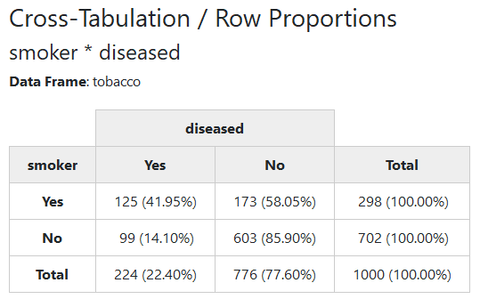
We’ll now use a sample data frame called tobacco, which is included in summarytools. We want to cross-tabulate two categorical variables: smoker and diseased.

Since markdown does not support multiline headings, we’ll show a rendered html version of the results:

print(ctable(tobacco$smoker, tobacco$diseased, prop = "r"), method = "render")

Note that we have to set the knitr chunk option results to “asis” for the results to appear as they should.

By default, ctable() shows row proportions. To show column or total proportions, use prop = "c" or prop = "t", respectively. To omit proportions, use prop = "n".

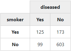
In the next example, we’ll create a simple “2 x 2” table (no proportions, no totals):

with(tobacco, 
     print(ctable(smoker, diseased, prop = 'n', totals = FALSE),
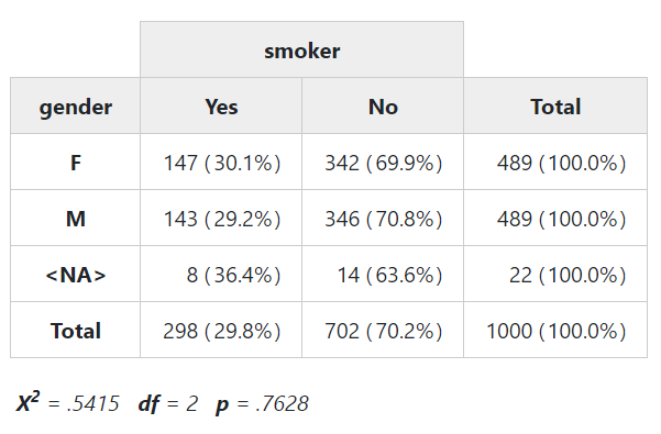
     headings = FALSE, method = "render"))

Chi-square results

To display chi-square results below the table, set the “chisq” parameter to TRUE. This time, instead of with(), we’ll use the %$% operator from the magrittr package, which works in a very similar fashion.

library(magrittr)
tobacco %$% ctable(gender, smoker, chisq = TRUE, headings = FALSE)

Note that a warning will be issued when at least one expected cell counts is lower than 5.

3 - descr() : Descriptive Univariate Stats

The descr() function generates common central tendency statistics and measures of dispersion for numerical data. It can handle single vectors as well as data frames, in which case it will ignore non-numerical columns (and display a message to that effect).

descr(iris, style = "rmarkdown")

Descriptive Statistics

iris
N: 150

	Petal.Length	Petal.Width	Sepal.Length	Sepal.Width
Mean	3.76	1.20	5.84	3.06
Std.Dev	1.77	0.76	0.83	0.44
Min	1.00	0.10	4.30	2.00
Q1	1.60	0.30	5.10	2.80
Median	4.35	1.30	5.80	3.00
Q3	5.10	1.80	6.40	3.30
Max	6.90	2.50	7.90	4.40
MAD	1.85	1.04	1.04	0.44
IQR	3.50	1.50	1.30	0.50
CV	0.47	0.64	0.14	0.14
Skewness	-0.27	-0.10	0.31	0.31
SE.Skewness	0.20	0.20	0.20	0.20
Kurtosis	-1.42	-1.36	-0.61	0.14
N.Valid	150.00	150.00	150.00	150.00
Pct.Valid	100.00	100.00	100.00	100.00

Transposing, Selecting Statistics

If your eyes/brain prefer seeing things the other way around, just use transpose = TRUE. Here, we also select only the statistics we wish to see, and specify headings = FALSE to avoid reprinting the same information as above.

We specify the stats we wish to report with the stats argument, which also accepts values “all”, “fivenum”, and “common”. See ?descr for a complete list of available statistics.

descr(iris, stats = "common", transpose = TRUE, headings = FALSE, style = "rmarkdown")

	Mean	Std.Dev	Min	Median	Max	N.Valid	Pct.Valid
Petal.Length	3.76	1.77	1.00	4.35	6.90	150.00	100.00
Petal.Width	1.20	0.76	0.10	1.30	2.50	150.00	100.00
Sepal.Length	5.84	0.83	4.30	5.80	7.90	150.00	100.00
Sepal.Width	3.06	0.44	2.00	3.00	4.40	150.00	100.00

4 - dfSummary() : Data Frame Summaries

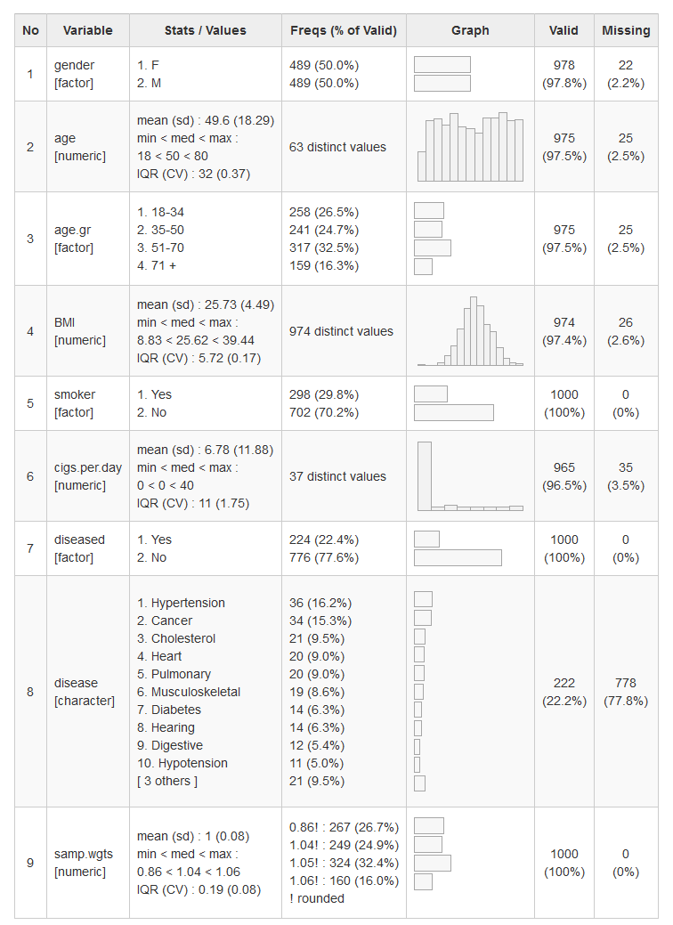
dfSummary() collects information about all variables in a data frame and displays it in a single legible table.

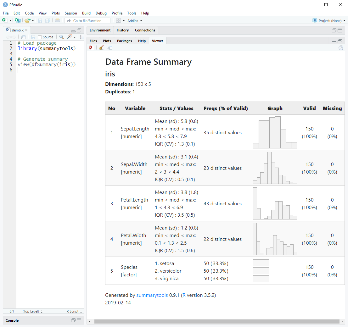
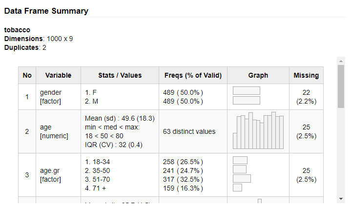
To generate a summary report and have it displayed in RStudio’s Viewer pane (or in the default Web browser if working outside RStudio), we simply do as follows:

library(summarytools)
view(dfSummary(iris))

Of course, it is also possible to use dfSummary() in Rmarkdown documents. It is usually a good idea to exclude a column or two, otherwise the table might be a bit too wide. For instance, since the Valid and NA columns are redundant, we can drop one of them.

dfSummary(tobacco, plain.ascii = FALSE, style = "grid", 
          graph.magnif = 0.75, valid.col = FALSE, tmp.img.dir = "/tmp")

While rendering html tables with view() doesn’t require it, here it is essential to specify tmp.img.dir. We’ll explain why further below.

Tidy Tables With tb()

When generating freq() or descr() tables, it is possible to turn the results into “tidy” tables with the use of the tb() function (think of tb as a diminutive for tibble). For example:

library(magrittr)
iris %>% descr(stats = "common") %>% tb()

## # A tibble: 4 x 8
##   variable      mean    sd   min   med   max n.valid pct.valid
##   <chr>        <dbl> <dbl> <dbl> <dbl> <dbl>   <dbl>     <dbl>
## 1 Petal.Length  3.76 1.77    1    4.35   6.9     150       100
## 2 Petal.Width   1.20 0.762   0.1  1.3    2.5     150       100
## 3 Sepal.Length  5.84 0.828   4.3  5.8    7.9     150       100
## 4 Sepal.Width   3.06 0.436   2    3      4.4     150       100

iris$Species %>% freq(cumul = FALSE, report.nas = FALSE) %>% tb()

## # A tibble: 3 x 3
##   value       freq   pct
##   <fct>      <dbl> <dbl>
## 1 setosa        50  33.3
## 2 versicolor    50  33.3
## 3 virginica     50  33.3

By definition, no total rows are part of tidy tables, and row.names are converted to regular columns.

Tidy Split-Group Statistics

Here are two examples of how lists created using stby() are transformed into tibbles. Notice how the order parameter affects the table’s row ordering:

grouped_freqs <- stby(data = tobacco$smoker, INDICES = tobacco$gender, 
                      FUN = freq, cumul = FALSE, report.nas = FALSE)
grouped_freqs %>% tb()

## # A tibble: 4 x 4
##   gender smoker  freq   pct
##   <fct>  <fct>  <dbl> <dbl>
## 1 F      Yes      147  15.0
## 2 F      No       342  35.0
## 3 M      Yes      143  14.6
## 4 M      No       346  35.4

grouped_freqs %>% tb(order = 2)

## # A tibble: 4 x 4
##   gender smoker  freq   pct
##   <fct>  <fct>  <dbl> <dbl>
## 1 F      Yes      147  15.0
## 2 M      Yes      143  14.6
## 3 F      No       342  35.0
## 4 M      No       346  35.4

grouped_descr <- stby(data = exams, INDICES = exams$gender, 
                      FUN = descr, stats = "common")
grouped_descr %>% tb()

## # A tibble: 12 x 9
##    gender variable   mean    sd   min   med   max n.valid pct.valid
##    <fct>  <chr>     <dbl> <dbl> <dbl> <dbl> <dbl>   <dbl>     <dbl>
##  1 Girl   economics  72.5  7.79  62.3  70.2  89.6      14      93.3
##  2 Girl   english    73.9  9.41  58.3  71.8  93.1      14      93.3
##  3 Girl   french     71.1 12.4   44.8  68.4  93.7      14      93.3
##  4 Girl   geography  67.3  8.26  50.4  67.3  78.9      15     100  
##  5 Girl   history    71.2  9.17  53.9  72.9  86.4      15     100  
##  6 Girl   math       73.8  9.03  55.6  74.8  86.3      14      93.3
##  7 Boy    economics  75.2  9.40  60.5  71.7  94.2      15     100  
##  8 Boy    english    77.8  5.94  69.6  77.6  90.2      15     100  
##  9 Boy    french     76.6  8.63  63.2  74.8  94.7      15     100  
## 10 Boy    geography  73   12.4   47.2  71.2  96.3      14      93.3
## 11 Boy    history    74.4 11.2   54.4  72.6  93.5      15     100  
## 12 Boy    math       73.3  9.68  60.5  72.2  93.2      14      93.3

grouped_descr %>% tb(order = 2)

## # A tibble: 12 x 9
##    gender variable   mean    sd   min   med   max n.valid pct.valid
##    <fct>  <chr>     <dbl> <dbl> <dbl> <dbl> <dbl>   <dbl>     <dbl>
##  1 Girl   economics  72.5  7.79  62.3  70.2  89.6      14      93.3
##  2 Boy    economics  75.2  9.40  60.5  71.7  94.2      15     100  
##  3 Girl   english    73.9  9.41  58.3  71.8  93.1      14      93.3
##  4 Boy    english    77.8  5.94  69.6  77.6  90.2      15     100  
##  5 Girl   french     71.1 12.4   44.8  68.4  93.7      14      93.3
##  6 Boy    french     76.6  8.63  63.2  74.8  94.7      15     100  
##  7 Girl   geography  67.3  8.26  50.4  67.3  78.9      15     100  
##  8 Boy    geography  73   12.4   47.2  71.2  96.3      14      93.3
##  9 Girl   history    71.2  9.17  53.9  72.9  86.4      15     100  
## 10 Boy    history    74.4 11.2   54.4  72.6  93.5      15     100  
## 11 Girl   math       73.8  9.03  55.6  74.8  86.3      14      93.3
## 12 Boy    math       73.3  9.68  60.5  72.2  93.2      14      93.3

The print() and view() Functions

summarytools has a generic print method, print.summarytools(). By default, its method argument is set to “pander”. One of the ways in which view() is useful is that we can use it to easily display html outputs in RStudio’s Viewer. The view() function simply acts as a wrapper around print.summarytools(), specifying method = 'viewer'. When used outside RStudio, method falls back to “browser” and the report is shown in the system’s default browser.

Using stby() to Ventilate Results

We can use stby() the same way as R’s base function by() with the four core summarytools functions. This returns a list-type object containing as many elements as there are categories in the grouping variable.

Why not just use by()? The reason is that by() creates objects of class “by()”, which have a dedicated print() method conflicting with summarytools’ way of printing list-type objects. Since print.by() can’t be redefined (as of CRAN policies), the sensible solution was to introduce a function that is essentially a clone of by(), except that the objects it creates have the class “stby”, allowing the desired flexibility.

Using the iris data frame, we will now display descriptive statistics by Species.

(iris_stats_by_species <- stby(data = iris, 
                               INDICES = iris$Species, 
                               FUN = descr, stats = c("mean", "sd", "min", "med", "max"), 
                               transpose = TRUE))

## Non-numerical variable(s) ignored: Species

Descriptive Statistics

iris
Group: Species = setosa
N: 50

	Mean	Std.Dev	Min	Median	Max
Petal.Length	1.46	0.17	1.00	1.50	1.90
Petal.Width	0.25	0.11	0.10	0.20	0.60
Sepal.Length	5.01	0.35	4.30	5.00	5.80
Sepal.Width	3.43	0.38	2.30	3.40	4.40

Group: Species = versicolor
N: 50

	Mean	Std.Dev	Min	Median	Max
Petal.Length	4.26	0.47	3.00	4.35	5.10
Petal.Width	1.33	0.20	1.00	1.30	1.80
Sepal.Length	5.94	0.52	4.90	5.90	7.00
Sepal.Width	2.77	0.31	2.00	2.80	3.40

Group: Species = virginica
N: 50

	Mean	Std.Dev	Min	Median	Max
Petal.Length	5.55	0.55	4.50	5.55	6.90
Petal.Width	2.03	0.27	1.40	2.00	2.50
Sepal.Length	6.59	0.64	4.90	6.50	7.90
Sepal.Width	2.97	0.32	2.20	3.00	3.80

To see an html version of these results, we simply use view() (also possible is to use print() with method = "viewer"): (results not shown)

view(iris_stats_by_species)
# or
print(iris_stats_by_species, method = "viewer")

A special situation occurs when we want grouped statistics for one variable only. Instead of showing several tables, each having one column, summarytools assembles everything into a single table:

data(tobacco)
with(tobacco, stby(BMI, age.gr, descr, 
                        stats = c("mean", "sd", "min", "med", "max")))

Descriptive Statistics

BMI by age.gr
Data Frame: tobacco
N: 258

	18-34	35-50	51-70	71 +
Mean	23.84	25.11	26.91	27.45
Std.Dev	4.23	4.34	4.26	4.37
Min	8.83	10.35	9.01	16.36
Median	24.04	25.11	26.77	27.52
Max	34.84	39.44	39.21	38.37

The transposed version looks like this:

	Mean	Std.Dev	Min	Median	Max
18-34	23.84	4.23	8.83	24.04	34.84
35-50	25.11	4.34	10.35	25.11	39.44
51-70	26.91	4.26	9.01	26.77	39.21
71 +	27.45	4.37	16.36	27.52	38.37

Using stby() With ctable()

This is a little trickier – the working syntax is as follows:

stby(list(x = tobacco$smoker, y = tobacco$diseased), tobacco$gender, ctable)
# or equivalently
with(tobacco, stby(list(x = smoker, y = diseased), gender, ctable))

Using dplyr::group_by() to Ventilate Results

To create grouped statistics with descr() or dfSummary(), it is possible to use dplyr’s group_by() as an alternative to stby(). Aside from the syntactic differences, one key distinction is that dplyr::group_by() considers NA values on the grouping variables as valid categories, albeit with a warning message suggesting to use forcats::fct_explicit_na to make NA’s explicit. The best way to go is simply to follow that advice:

library(dplyr)
tobacco$gender <- forcats::fct_explicit_na(tobacco$gender)
tobacco %>% group_by(gender) %>% descr(stats = "fivenum")

## Non-numerical variable(s) ignored: gender, age.gr, smoker, diseased, disease

Descriptive Statistics

tobacco
Group: gender = F
N: 489

	age	BMI	cigs.per.day	samp.wgts
Min	18.00	9.01	0.00	0.86
Q1	34.00	22.98	0.00	0.86
Median	50.00	25.87	0.00	1.04
Q3	66.00	29.48	10.50	1.05
Max	80.00	39.44	40.00	1.06

Group: gender = M
N: 489

	age	BMI	cigs.per.day	samp.wgts
Min	18.00	8.83	0.00	0.86
Q1	34.00	22.52	0.00	0.86
Median	49.50	25.14	0.00	1.04
Q3	66.00	27.96	11.00	1.05
Max	80.00	36.76	40.00	1.06

Group: gender = (Missing)
N: 22

	age	BMI	cigs.per.day	samp.wgts
Min	19.00	20.24	0.00	0.86
Q1	36.00	24.97	0.00	1.04
Median	55.50	27.16	0.00	1.05
Q3	64.00	30.23	10.00	1.05
Max	80.00	32.43	28.00	1.06

Using summarytools in Rmarkdown Documents

As we have seen, summarytools can generate both text/markdown and html results. Both types of outputs can be used in Rmarkdown documents. The vignette Recommendations for Using summarytools With Rmarkdown provides good guidelines, but here are a few tips to get started:

Always set the knitr chunk option results = 'asis'. You can do this on a chunk-by-chunk basis, but it is easier to just set it globally in a “setup” chunk:

    knitr::opts_chunk$set(echo = TRUE, results = 'asis')

Refer to this page to learn more about knitr’s options.

To get better results when generating html output with method = 'render', set up your .Rmd document so that it includes summarytools’ css. The st_css() function makes this very easy.

Initial Setup – Example

# ---
# title: "RMarkdown using summarytools"
# output: html_document
# ---
#
# ```{r setup, include=FALSE}
# library(knitr)
# opts_chunk$set(comment = NA, prompt = FALSE, cache = FALSE, results = 'asis')
# library(summarytools)
# st_options(plain.ascii = FALSE,          # This is a must in Rmd documents
#            style = "rmarkdown",          # idem
#            dfSummary.varnumbers = FALSE, # This keeps results narrow enough
#            dfSummary.valid.col = FALSE)  # idem
#```
#
# ```{r, echo=FALSE}
# st_css()
# ```

Since results = 'asis' can conflict with other packages’ way of generating results, it is sometimes best to use it for individual chunks only.

Managing Lengthy dfSummary() Outputs in Rmarkdown Documents

For data frames containing numerous variables, we can use the max.tbl.height argument to wrap the results in a scrollable window having the specified height, in pixels. For instance:

print(dfSummary(tobacco, valid.col = FALSE, graph.magnif = 0.75), 
      max.tbl.height = 300, method = "render")

Writing Output to Files

We can use the file argument with print() or view() to indicate that we want to save the results in a file, be it html, Rmd, md, or just plain text (txt). The file extension indicates to summarytools what type of file should be generated.

view(iris_stats_by_species, file = "~/iris_stats_by_species.html")

Appending Output Files

The append argument allows adding content to existing files generated by summarytools. This is useful if you want to include several statistical tables in a single file. It is a quick alternative to creating an .Rmd document.

Global options

The following options can be set with st_options():

General Options

Option name	Default	Note
style	“simple”	Set to “rmarkdown” in .Rmd documents
plain.ascii	TRUE	Set to FALSE in .Rmd documents
round.digits	2	Number of decimals to show
headings	TRUE	Formerly “omit.headings”
footnote	“default”	Personalize, or set to NA to omit
display.labels	TRUE	Show variable / data frame labels in headings
bootstrap.css (*)	TRUE	Include Bootstrap 4 css in html outputs
custom.css	NA	Path to your own css file
escape.pipe	FALSE	Useful for some Pandoc conversions
subtitle.emphasis	TRUE	Controls headings formatting
lang	“en”	Language (always 2-letter, lowercase)

(*) Set to FALSE in Shiny apps

Function-Specific Options

Option name	Default	Note
freq.totals	TRUE	Display totals row in freq()
freq.report.nas	TRUE	Display row and “valid” columns
ctable.prop	“r”	Display row proportions
ctable.totals	TRUE	Show marginal totals
descr.stats	“all”	“fivenum”, “common” or vector of stats
descr.transpose	FALSE
descr.silent	FALSE	Hide console messages
dfSummary.varnumbers	TRUE	Show variable numbers in 1st col.
dfSummary.labels.col	TRUE	Show variable labels when present
dfSummary.graph.col	TRUE	Show graphs
dfSummary.valid.col	TRUE	Include the Valid column in the output
dfSummary.na.col	TRUE	Include the Missing column in the output
dfSummary.graph.magnif	1	Zoom factor for bar plots and histograms
dfSummary.silent	FALSE	Hide console messages
tmp.img.dir	NA	Directory to store temporary images

Examples

st_options()                      # display all global options values
st_options('round.digits')        # display the value of a specific option
st_options(style = 'rmarkdown')   # change one or several options' values
st_options(footnote = NA)         # Turn off the footnote on all outputs.
                                  # This option was used prior to generating
                                  # the present document.

Overriding formatting attributes

When a summarytools object is created, its formatting attributes are stored within it. However, you can override most of them when using the print() method or the view() function.

Overriding Function-Specific Arguments

Argument	freq	ctable	descr	dfSummary
style	x	x	x	x
round.digits	x	x	x
plain.ascii	x	x	x	x
justify	x	x	x	x
headings	x	x	x	x
display.labels	x	x	x	x
varnumbers				x
labels.col				x
graph.col				x
valid.col				x
na.col				x
col.widths				x
totals	x	x
report.nas	x
display.type	x
missing	x
split.tables	x	x	x	x
caption	x	x	x	x

Overriding Headings Content

Argument	freq	ctable	descr	dfSummary
Data.frame	x	x	x	x
Data.frame.label	x	x	x	x
Variable	x	x	x
Variable.label	x	x	x
Group	x	x	x	x
date	x	x	x	x
Weights	x		x
Data.type	x
Row.variable		x
Col.variable		x

Example

Here’s an example in which we override 3 function-specific arguments, and one element of the heading:

(age_stats <- freq(tobacco$age.gr))

Frequencies

tobacco$age.gr
Type: Factor

	Freq	% Valid	% Valid Cum.	% Total	% Total Cum.
18-34	258	26.46	26.46	25.80	25.80
35-50	241	24.72	51.18	24.10	49.90
51-70	317	32.51	83.69	31.70	81.60
71 +	159	16.31	100.00	15.90	97.50
<NA>	25			2.50	100.00
Total	1000	100.00	100.00	100.00	100.00

print(age_stats, report.nas = FALSE, totals = FALSE, display.type = FALSE,
      Variable.label = "Age Group")

Frequencies

tobacco$age.gr
Label: Age Group

	Freq	%	% Cum.
18-34	258	26.46	26.46
35-50	241	24.72	51.18
51-70	317	32.51	83.69
71 +	159	16.31	100.00

Note that the original attributes are still part of the age_stats object, left unchanged.

Order of Priority for Options / Parameters

Options overridden explicitly in print() or view() have precedence
Options specified as explicit arguments to freq() / ctable() / descr() / dfSummary() come second
Global options set with st_options come third

Customizing looks with CSS

summarytools uses RStudio’s htmltools package and version 4 of Bootstrap’s cascading stylesheets.

It is possible to include your own css if you wish to customize the look of the output tables. See ?print.summarytools for all the details, but here is a quick example.

Say you need to make the font size really really small. For this, you would create a .css file - let’s call it “custom.css” - containing a class definition such as the following:

.tiny-text {
  font-size: 8px;
}

Then, to apply it to a summarytools object and display it in your browser:

view(dfSummary(tobacco), custom.css = 'path/to/custom.css', 
     table.classes = 'tiny-text')

To display a smaller table that is not that small, you can use the provided css class st-small.

Working with Shiny apps

To include summarytools functions in Shiny apps, it is recommended that you:

set bootstrap.css = FALSE to avoid interacting with the app’s layout
omit headings by setting the global option headings = FALSE
adjust the size of the graphs in dfSummary() using the dfSummary.graph.magnif global option
if dfSummary() outputs are too wide, try omitting a column or two (valid.col and varnumbers, for instance)
if needed, set the column widths manually with the col.widths parameter of the print() method or the view() function

print(dfSummary(somedata, graph.magnif = 0.8), 
      method = 'render',
      headings = FALSE,
      bootstrap.css = FALSE)

Graphs in Markdown dfSummaries

When generating markdown (as opposed to html) summaries in an .Rmd document, three elements are needed to display proper png graphs:

1 - plain.ascii is FALSE
2 - style is “grid”
3 - tmp.img.dir is defined

Why the third element? Although R makes it really easy to create temporary files and directories, they do have long pathnames, especially on Windows. Combine this with the fact that Pandoc currently determines the final (rendered) column widths by counting characters, including those of pathnames pointing to images. What we get is… some issues of proportion (!).

At this time, there seems to be only one solution around this problem: cut down on characters in pathnames. So instead of this:

+-----------+-------------------------------------------------------------------------+---------+
| Variable  | Graph                                                                   | Valid   |
+===========+=========================================================================+=========+
| gender\   | ![](C:/Users/johnny/AppData/Local/Temp/RtmpYRgetx/file5aa4549a4d71.png) | 978\    |
| [factor]  |                                                                         | (97.8%) |
+----+---------------+----------------------------------------------------------------+---------+

…we aim for this:

+---------------+----------------------+---------+
| Variable      | Graph                | Valid   |
+===============+======================+=========+
| gender\       | ![](/tmp/ds0001.png) | 978\    |
| [factor]      |                      | (97.8%) |
+---------------+----------------------+---------+

Now CRAN policies are really strict when it comes to writing content in the user directories, or anywhere outside R’s temporary zone (for good reasons). So we need to let the users set this location themselves, therefore implicitly consenting to content being written outside R’s temporary zone.

On Mac OS and Linux, using “/tmp” makes a lot of sense: it’s short, and it’s self-cleaning. On Windows, there is no such convenient directory, so we need to pick one – be it absolute (“/tmp”) or relative (“img”, or simply “.”). Two things are to be kept in mind: it needs to be short (5 characters max) and we need to clean it up manually.

Translations

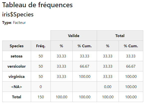
It is now possible to select the language used in the outputs. The following languages are available: English (en - default), French (fr), Spanish (es), Portuguese (pt), Turkish (tr), and Russian (ru). With the R community’s involvement, I believe we can add several more as time goes on.

Switching Languages

To switch languages, simply use

st_options(lang = "fr")

Any function will now produce outputs using that language:

view(freq(iris$Species))

The language used for producing the object is stored within it as an attribute. This is to avoid problems when switching languages between the moment the object is stored, and the moment at which it is printed.

Non-UTF-8 Locales

On most Windows systems, it will be necessary to change the LC_CTYPE element of the locale settings if the character set is not included in the current locale. For instance, in order to get good results – or rather, any results at all – with the Russian language in a “latin1” environment, we’ll need to do this:

Sys.setlocale("LC_CTYPE", "russian")
st_options(lang = 'ru')

Then, to go back to default settings:

Sys.setlocale("LC_CTYPE", "")
st_options(lang = "en")

Defining and Using Custom Translations

Using the function use_custom_lang(), it is possible to add your own set of translations. To achieve this, simply download the template csv file from this page, customize the +/- 70 items, and call use_custom_lang(), giving it as sole argument the path to the csv file you’ve created. Note that such custom translations will not persist across R sessions. This means that you should always have this csv file handy.

Defining Specific Keywords

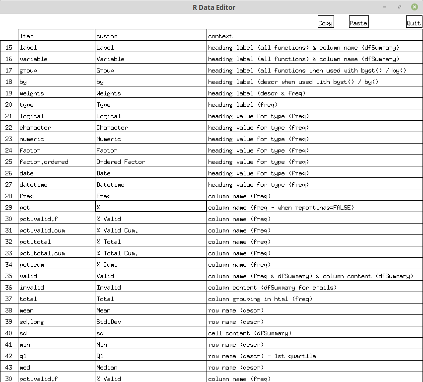
Sometimes, all you might want to do is change just a few keywords – say you would rather have “N” instead of “Freq” in the title row of freq() tables. No need to create a full custom language for that. Rather, use define_keywords(). Calling this function without any arguments will bring up, on systems that support graphical devices (the vast majority, that is), an editable window allowing the modify only the desired items.

After closing the edit window, you will be offered to export the resulting “custom language” into a .csv file that can be imported later on with use_custom_lang().

Note that it is also possible to define one or several keywords using arguments. For the list of all possible keywords to define, see ?define_keywords. For instance:

define_keywords(freq = "N")

Latest Changes and Improvements

As stated earlier, version 0.9 brought many improvements to summarytools. Here are the key elements:

Translations
Improved printing of list objects
- Objects of class “stby” are automatically printed in the console with optimal results; no more need for view(x, method = "pander"); simply use stby() instead of by()
- Regular lists containing summarytools objects can also be printed with optimal results simply by calling print(x) (as opposed to “stby” objects, their automatic printing will not be optimal; that being said, freq() now accepts data frames as its first argument, so the need for lapply() is greatly reduced)
Easier management of global settings with st_options()
- st_options() now has as many parameters as there are options to set, making it possible to set all options with only one function call; legacy way of setting options is still supported
- Several global options were added, with a focus on simplifying Rmarkdown document creation
Changes to freq()
- As mentioned earlier, the function now accepts data frames as its main argument; this makes practically obsolete the use of lapply() with it
Improved outputs when using stby()
Changes to ctable()
- Fully supports stby()
- Improved number alignment
- Added “chisq” parameter
Changes to descr()
- For the stats argument, Values “fivenum” and “common” are now allowed, the latter representing the collection of mean, sd, min, med, max, n.valid, and pct.valid
- Improved outputs when using stby()
- The variable used for weights (if any) is removed automatically from the data so no stats are produced for it
Changes to dfSummary()
- Now fully compatible with Rmarkdown
- Number of columns is now included in the heading section
- Number of duplicated rows is also shown in the heading section
- Bar plots now more accurately reflect counts, as they are not stretched across table cells (this allows the comparison of frequencies across variables)
- Columns with particular content (unary/binary, integer sequences, UPC/EAN codes) are treated differently; more relevant information is displayed, while irrelevant information is hidden
- For html outputs, a new parameter col.widths can be used to set the width of the resulting table’s columns; this addresses an issue with some graphs not being shown at the desired magnification level (although much effort has been put into improving this as well)
- max.tbl.height parameter added

Stay Up-to-date

For a preview of what’s coming in the next release, see the development branch.

Final notes

The package comes with no guarantees. It is a work in progress and feedback / feature requests are welcome. Just send me an email (dominic.comtois (at) gmail.com), or open an issue if you find a bug or wish to submit a feature request.

Also, the package grew significantly larger, and maintaining it all by myself is time consuming. If you would like to contribute, please get in touch, I’d greatly appreciate the help.

jrgant/summarytools

summarytools

What is summarytools?

Latest Improvements

How to install

From GitHub

From CRAN

The Four Core Functions

1 - freq() : Frequency Tables

Frequencies

Subsetting Rows in Frequency Tables

Generating Several Frequency Tables at Once

2 - ctable() : Cross-Tabulations

Chi-square results

3 - descr() : Descriptive Univariate Stats

Descriptive Statistics

Transposing, Selecting Statistics

4 - dfSummary() : Data Frame Summaries

Tidy Tables With tb()

Tidy Split-Group Statistics

The print() and view() Functions

Using stby() to Ventilate Results

Descriptive Statistics

Descriptive Statistics

Using stby() With ctable()

Using dplyr::group_by() to Ventilate Results

Descriptive Statistics

Using summarytools in Rmarkdown Documents

Initial Setup – Example

Managing Lengthy dfSummary() Outputs in Rmarkdown Documents

Writing Output to Files

Appending Output Files

Global options

General Options

Function-Specific Options

Examples

Overriding formatting attributes

Overriding Function-Specific Arguments

Overriding Headings Content

Example

Frequencies

Frequencies

Order of Priority for Options / Parameters

Customizing looks with CSS

Working with Shiny apps

Graphs in Markdown dfSummaries

Translations

Switching Languages

Non-UTF-8 Locales

Defining and Using Custom Translations

Defining Specific Keywords

Latest Changes and Improvements

Stay Up-to-date

Final notes