l0g1c-80m8/3d-motion-planning

Motion planning of a drone in a simulated map of San Francisco!

Project: 3D Motion Planning

---

Overview

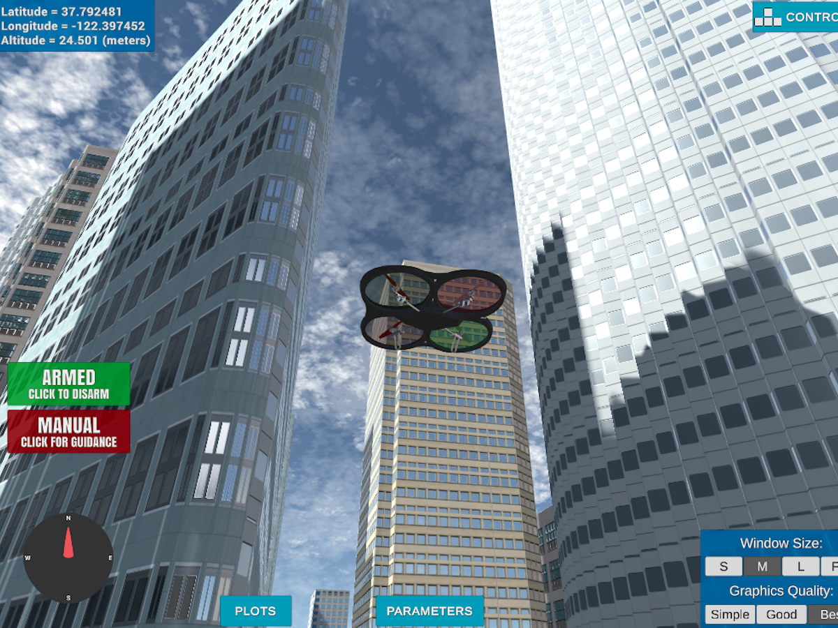
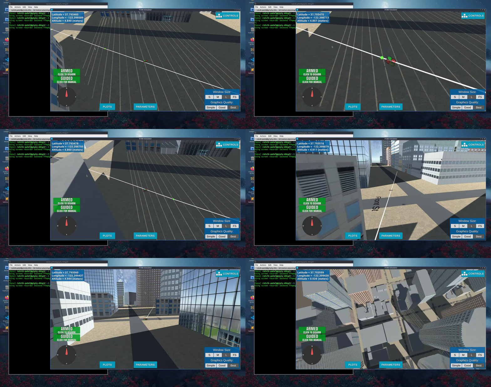
This project aims to simulate a mission of a drone in an urban environment. The steps undertaken to achieve this are follows:

1. Load the 2.5D map in the colliders.csv file describing the environment.
2. Discretize the environment into a grid or graph representation.
3. Define the start and goal locations.
4. Perform a search using A* or other search algorithm.
5. Use a collinearity test or ray tracing method (like Bresenham) to remove unnecessary waypoints.
6. Return waypoints in local ECEF coordinates (format for self.all_waypoints is [N, E, altitude, heading], where the drone’s start location corresponds to [0, 0, 0, 0].

The Starter Code

This project is forked from FCND-Motion-Planning project. This project completes the partial implementation of its fork.

Functionality of motion_planning.py and planning_utils.py

The motion_planning.py contains the main class MotionPlanning of the script that communicates with the simulator and starts the execution. MotionPlanning is a finite state machine containing all the callback methods local_position_callback, velocity_callback and state_callback which are executed when the position, velocity or the state change respectively. The state_callback handles which state transition to make and calls the appropriate method.

There is a special method plan_path which houses the implementation required to perform steps 1. to 6. stated above. A lot of this functionality has been defined in planning_utils.py like the implementation of A* search, bresenham ray-tracing, etc. Additionally, there are general_utils.py and constants.py files that facilitate declaration of general utils or common data used by the main two files.

The Simulation environment

Here is a lovely picture of downtown San Francisco environment from above:

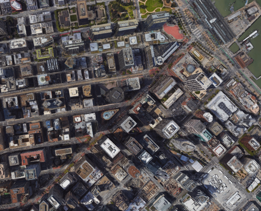
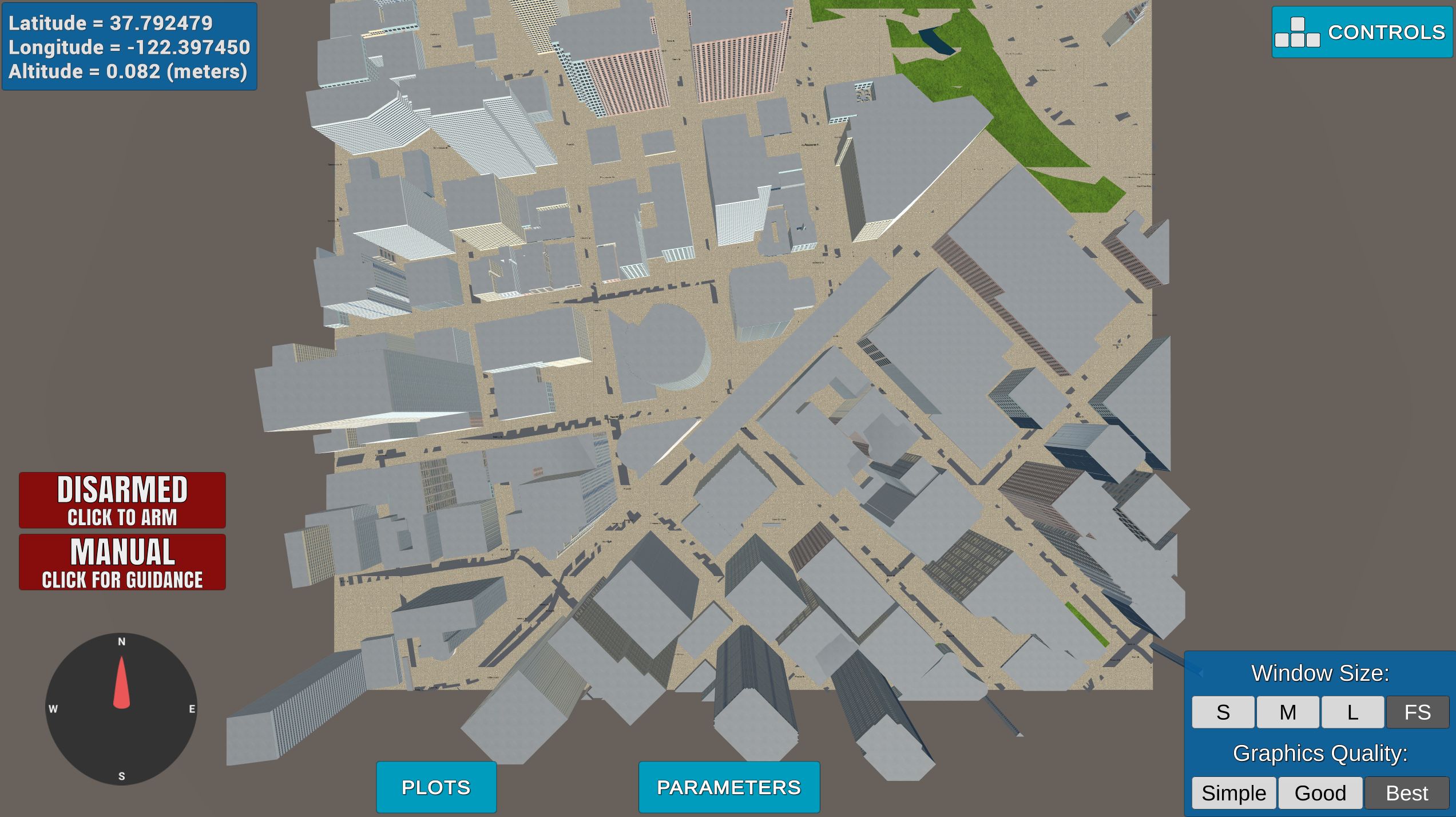
And here is the equivalent view of the simulation environment from above:

The Path Planning Algorithm

1. Set global home position

Read the first line of the csv file using general_utils.read_line_from_file, parse the line to extract lat0 and lon0 values and convert them to float in general_utils.parse_lat_lon_alt(). Use self.set_home_position() method to set global home.

2. Set current local position

Use global_to_local() to get northing, easting values from longitude and latitude coordinates.

3. Set grid start position from local position

Use planning_utils.relative_grid_pose() to offset the starting position in the grid correctly.

4. Set grid goal position from geodetic coords

Use planning_utils.get_grid_goal() to get a far, medium or nearby value in the grid.

5. Search algorithm

Implement the search algorithm to model produce a naive path on the grid cells.

6. Cull waypoints

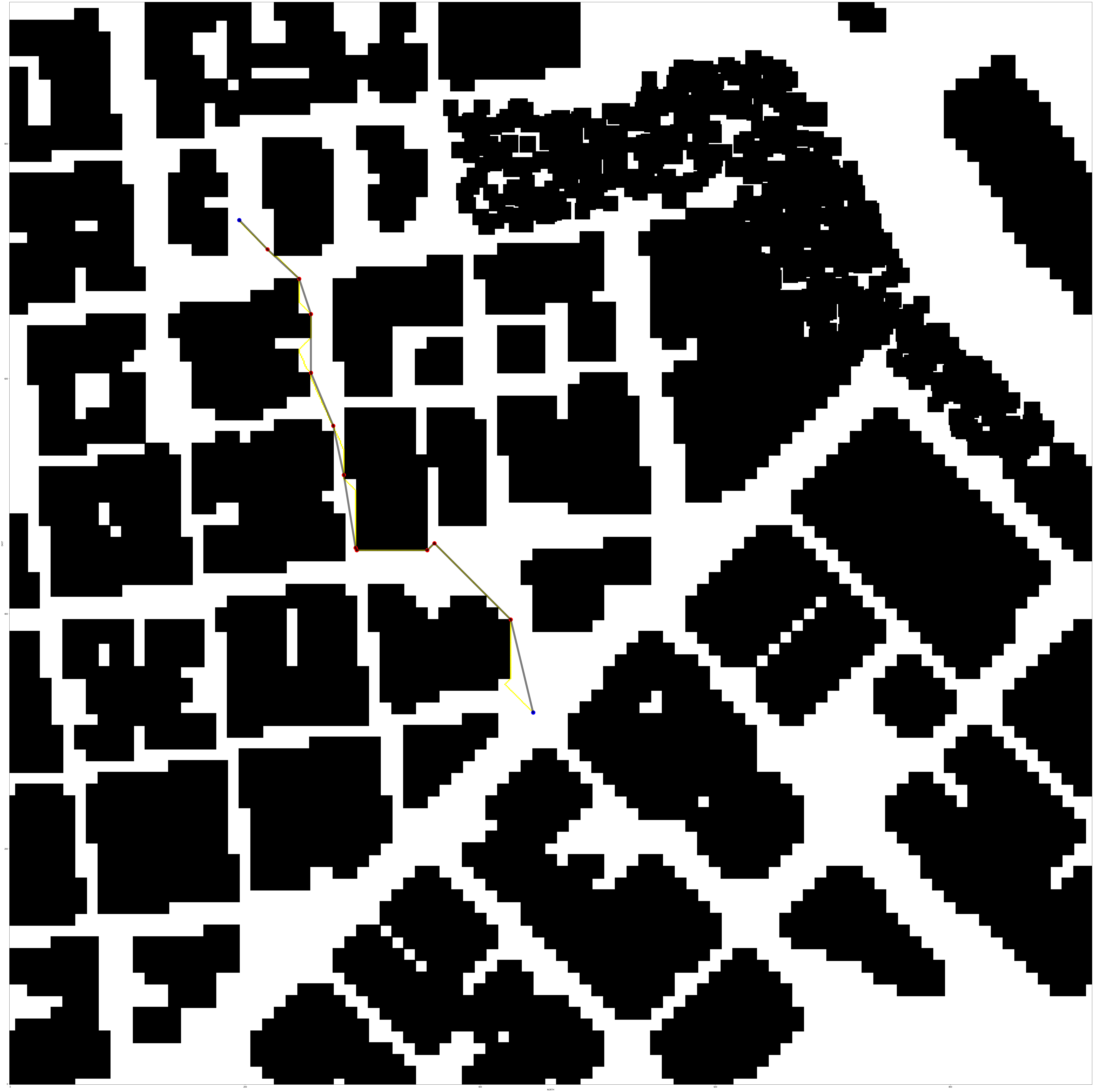
Use the planning_utils.prune_path() method implementing the Bresenham ray-tracing algorithm to remove unnecessary waypoints from the naive path.

Results

Key:

• Blue points are start and goal nodes.
• Yellow points are waypoints generated by the search algorithm.
• Red points are waypoints after pruning by Bresenham's ray-tracing algorithm.
• Thicker (Black/Blue) lines make up the paths connecting the waypoints.

Planning with RRT:

Planning with A*:

Demo simulation run

Tasks

• Implement with .
• Implement with D* Lite.
• Implement with .
• Implement with Probabilistic Roadmap.
• Implement as an Problem.