➡️ ESHG poster is available here.
ℹ️ bGWAS has been updated to version 1.0.2.
Check the NEWS to learn more about what has been modified!
Note: some Prior GWASs have been removed, you can find more details
here.
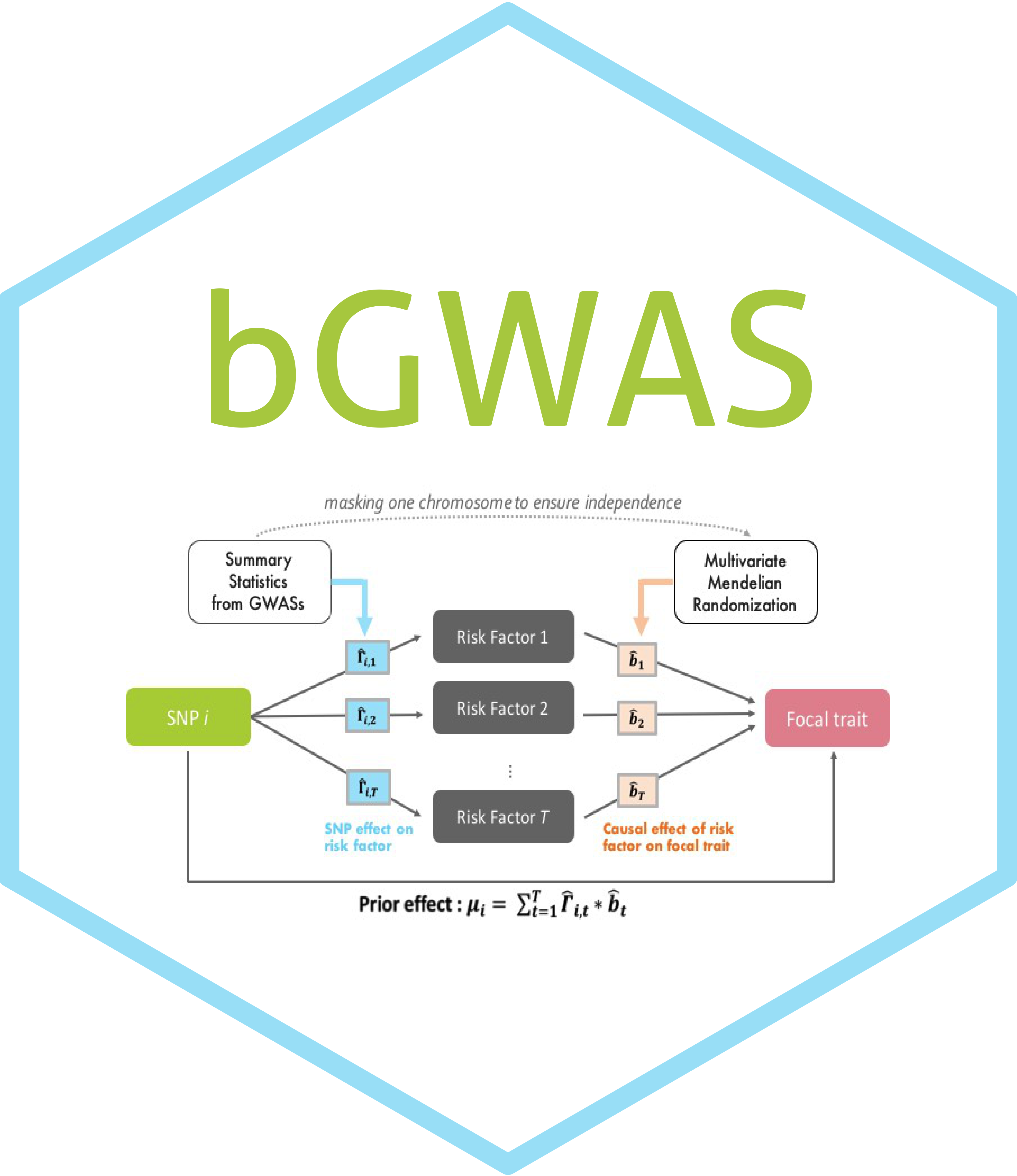
bGWAS is an R-package to perform a Bayesian GWAS (Genome Wide
Association Study), using summary statistics from a conventional GWAS as
input. The aim of the approach is to increase power by leveraging
information from related traits and by comparing the observed Z-scores
from the focal phenotype (provided as input) to prior effects. These
prior effects are directly estimated from publicly available GWASs
(currently, a set of 38 studies, last update 20-08-2019 - hereinafter
referred to as “prior GWASs” or “risk factors”). Only prior GWASs having
a significant causal effect on the focal phenotype, identified using a
multivariable Mendelian Randomization (MR) approach, are used to
calculate the prior effects. Causal effects are estimated masking the
focal chromosome to ensure independence, and the prior effects are
estimated as described in the figure below.

Observed and prior effects are compared using Bayes Factors. Significance is assessed by calculating the probability of observing a value larger than the observed BF (P-value) given the prior distribution. This is done by decomposing the analytical form of the BFs and using an approximation for most BFs to make the computation faster. Prior, posterior and direct effects, alongside BFs and p-values are returned. Note that prior, posterior and direct effects are estimated on the Z-score scale, but are automatically rescaled to beta scale if possible.
The principal functions available are:
-
bGWAS()
main function that calculates prior effects from prior GWASs, compares them to observed Z-scores and returns an object of class bGWAS -
list_priorGWASs()
directly returns information about the prior GWASs that can be used to calculate prior effects -
select_priorGWASs()
allows a quick selection of prior GWASs (to include/exclude specific studies when calculating prior effects) -
extract_results_bGWAS()
returns results (prior, posterior and direct estimate / standard-error + p-value from BF for SNPs) from an object of class bGWAS -
manhattan_plot_bGWAS()
creates a Manhattan Plot from an object of class bGWAS -
extract_MRcoeffs_bGWAS()
returns multivariable MR coefficients (1 estimate using all chromosomes + 22 estimates with 1 chromosome masked) from an object of class bGWAS -
coefficients_plot_bGWAS()
creates a Coefficients Plot (causal effect of each prior GWASs on the focal phenotype) from an object of class bGWAS -
heatmap_bGWAS()
creates a heatmap to represent, for each significant SNP, the contribution of each prior GWAS to the estimated prior effect from an object of class bGWAS
All the functions available and more details about their usage can be found in the manual.
You can install the current version of bGWAS with:
# Directly install the package from github
# install.packages("remotes")
remotes::install_github("n-mounier/bGWAS")
library(bGWAS)
## Warning: package 'dplyr' was built under R version 3.6.2
To run the analysis with bGWAS two inputs are needed:
Can be a regular (space/tab/comma-separated) file or a gzipped file
(.gz) or a data.frame. Must contain the following columns, which can
have alternative names:
SNP-identifier: rs or rsid, snp, snpid, rnpid
Alternate (effect) allele: a1 or alt, alts
Reference allele: a2 or a0, ref
Z-statistics: z or Z, zscore
If the Z-statistics is not present, it will be automatically calculated from effect size and standard error, in which case the following columns should be provided:
Effect-size: b or beta, beta1
Standard error: se or std
If you want the prior/posterior/corrected effects to be rescaled, please make sure to provide effect sizes and standard errors instead of (or in addition to) Z-statistics.
These files should be downloaded separately and stored in ~/ZMatrices
or in the folder specified when launching the analysis. These files
contains the Z-scores for all prior GWASs :
ZMatrix_MR.csv.gz: Z-scores (strong instruments only) used for
multivariable MR,
ZMatrix_Full.csv.gz: Z-scores (all SNPs) used to calculate the prior
Z-scores,
AvailableStudies.tsv: A file containing information about the prior
GWASs available.
You can download these files using this link or following the instructions below. Please note that your input GWAS will be merged with the Z-Matrix files (using rsid and alleles to align effects), and that the results reported will use the Z-Matrix files chr:pos information (GRCh37 - since UK10K data has been used to imputed the prior GWASs).
- On UNIX/MACOSX, from a terminal:
wget https://drive.switch.ch/index.php/s/jvSwoIxRgCKUSI8/download -O ZMatrices.tar.gz
tar xzvf ZMatrices.tar.gz
If you want to use your own set of prior GWASs, please have a look here to see how you can modify the files.
Before running your analysis, you can select the prior GWASs you want to
include. You can use the function list_priorGWASs() to get some
information about the prior GWASs available.
You should remove traits that by definition are not independent from
your trait of interest. For example, before analysing BMI results, make
sure to exclude “Height” from the prior GWASs used. You can use the
function select_priorGWASs() to automatically exclude/include some
traits or some files. You should also check for sample overlap, and
remove prior GWASs that come from the same consortium as your data. If
there are individuals in common between your conventional GWAS and prior
GWASs, it might induce some bias.
# Obtain the list of prior GWASs
AllStudies = list_priorGWASs()
# Select only the ones for specific traits
# select_priorGWASs will return the IDs of the files that are kept
MyStudies = select_priorGWASs(include_traits=c("Heart Rate", "Body Mass Index", "Smoking"))
# Match these IDs against the ones in the list of prior GWASs
AllStudies[AllStudies$ID %in% MyStudies, ]
## # A tibble: 6 x 10
## File
## <chr>
## 1 All_ancestries_SNP_gwas_mc_merge_nogc.tbl.uniq.gz
## 2 META_STAGE1_GWASHR_SUMSTATS.txt
## 3 tag.cpd.tbl.gz
## 4 tag.evrsmk.tbl.gz
## 5 tag.former.tbl.gz
## 6 tag.logonset.tbl.gz
## Name ID Trait Consortium
## <chr> <dbl> <chr> <chr>
## 1 Body Mass Index (GIANT) 1 Body Mass Index GIANT
## 2 Heart Rate (HRgene) 23 Heart Rate HRgene
## 3 Smoking - cigarettes per day (TAG) 35 Smoking TAG
## 4 Smoking - ever smoked (TAG) 36 Smoking TAG
## 5 Smoking - former smoker (TAG) 37 Smoking TAG
## 6 Smoking - age of onset (TAG) 38 Smoking TAG
## Reference Download Remarks N_SNPs N_Instruments
## <chr> <chr> <chr> <dbl> <dbl>
## 1 https://www.ncb… https://portals.broad… <NA> 6.81e6 10052
## 2 https://www.ncb… http://walker05.u.hpc… <NA> 6.81e6 3229
## 3 https://www.ncb… https://www.med.unc.e… Other GWAS Data … 6.63e6 558
## 4 https://www.ncb… https://www.med.unc.e… Other GWAS Data … 6.78e6 94
## 5 https://www.ncb… https://www.med.unc.e… Other GWAS Data … 6.78e6 184
## 6 https://www.ncb… https://www.med.unc.e… Other GWAS Data … 6.77e6 34
- Example A
# Using a small GWAS (400,000 SNPs, Timmers et al data - stored as a data.frame)
# Please, not that this example is only for illustration, the method is designed
# to be used genome-wide, and using such a low number of SNPs can not yield
# interpretable results.
data("SmallGWAS_Timmers2019")
MyStudies = select_priorGWASs(include_traits=c("Blood Pressure", "Education"),
include_files=c("cardiogram_gwas_results.txt", "All_ancestries_SNP_gwas_mc_merge_nogc.tbl.uniq.gz"))
# 6 Prior GWASs used
list_priorGWASs(MyStudies)[,c("Name", "Trait", "Reference")]
## # A tibble: 6 x 3
## Name Trait
## <chr> <chr>
## 1 Body Mass Index (GIANT) Body Mass Index
## 2 Coronary Artery Disease (CARDIoGRAM) Coronary Artery Disease
## 3 Years of Schooling (SSGAC) Education
## 4 Systolic Blood Pressure (ICBP) Blood Pressure
## 5 Diastolic Blood Pressure (ICBP) Blood Pressure
## 6 College Completion (SSGAC) Education
## Reference
## <chr>
## 1 https://www.ncbi.nlm.nih.gov/pubmed/25673413
## 2 https://www.ncbi.nlm.nih.gov/pubmed/21378990
## 3 https://www.ncbi.nlm.nih.gov/pubmed/27225129
## 4 https://www.ncbi.nlm.nih.gov/pubmed/21909115
## 5 https://www.ncbi.nlm.nih.gov/pubmed/21909115
## 6 https://www.ncbi.nlm.nih.gov/pubmed/23722424
A = bGWAS(name="Test_UsingSmallDataFrame",
          GWAS = SmallGWAS_Timmers2019,
          prior_studies = MyStudies,
          stepwise_threshold = 0.05)
# MR instruments will be selected using default parameter (1e-6) and distance-pruned (500Kb),
# MR will be performed using a threshold of 0.05 to select studies, and the default shrinkage thresholds (1) will be used,
# A subset of prior GWASs (MyStudies) will be used, and only the ones with at least 3 strong instruments will be kept to be tested and create the prior,
# Significant SNPs will be identified using default parameters (p<5e-8) and distance-pruned (500kb),
# No file will be saved.- Example B
# Using a GWAS from our list our prior GWASs
# Using all other (37) GWASs to built the prior
MyGWAS = 3
list_priorGWASs(MyGWAS)[, c("Name", "Trait", "Reference")]
## # A tibble: 1 x 3
## Name Trait
## <chr> <chr>
## 1 Coronary Artery Disease (CARDIoGRAM) Coronary Artery Disease
## Reference
## <chr>
## 1 https://www.ncbi.nlm.nih.gov/pubmed/21378990
B = bGWAS(name = "Test_UsingGWASfromPriorGWASs",
         GWAS = MyGWAS)
# MR instruments will be selected using default parameters,
# MR will be performed using default parameters (stepwise selection / shrinkage threshold)
# All Prior GWASs except the one use as "GWAS" will be used to create the prior,
# Significant SNPs will be identified using default parameters (p<5e-8) and distance-pruned (500kb)
# No file will be saved.bGWAS() returns an object of class “bGWAS” than can be handled in
R.
class(A)## [1] "bGWAS"
print(A)## -_-_-_-_-_-_-_-_-_-_-_-_-_-_-_
##
## Analysis : "Test_UsingSmallDataFrame"
## bGWAS performed on 286,807 SNPs
##
## -_-_-_-_-_-_-_-_-_-_-_-_-_-_-_
##
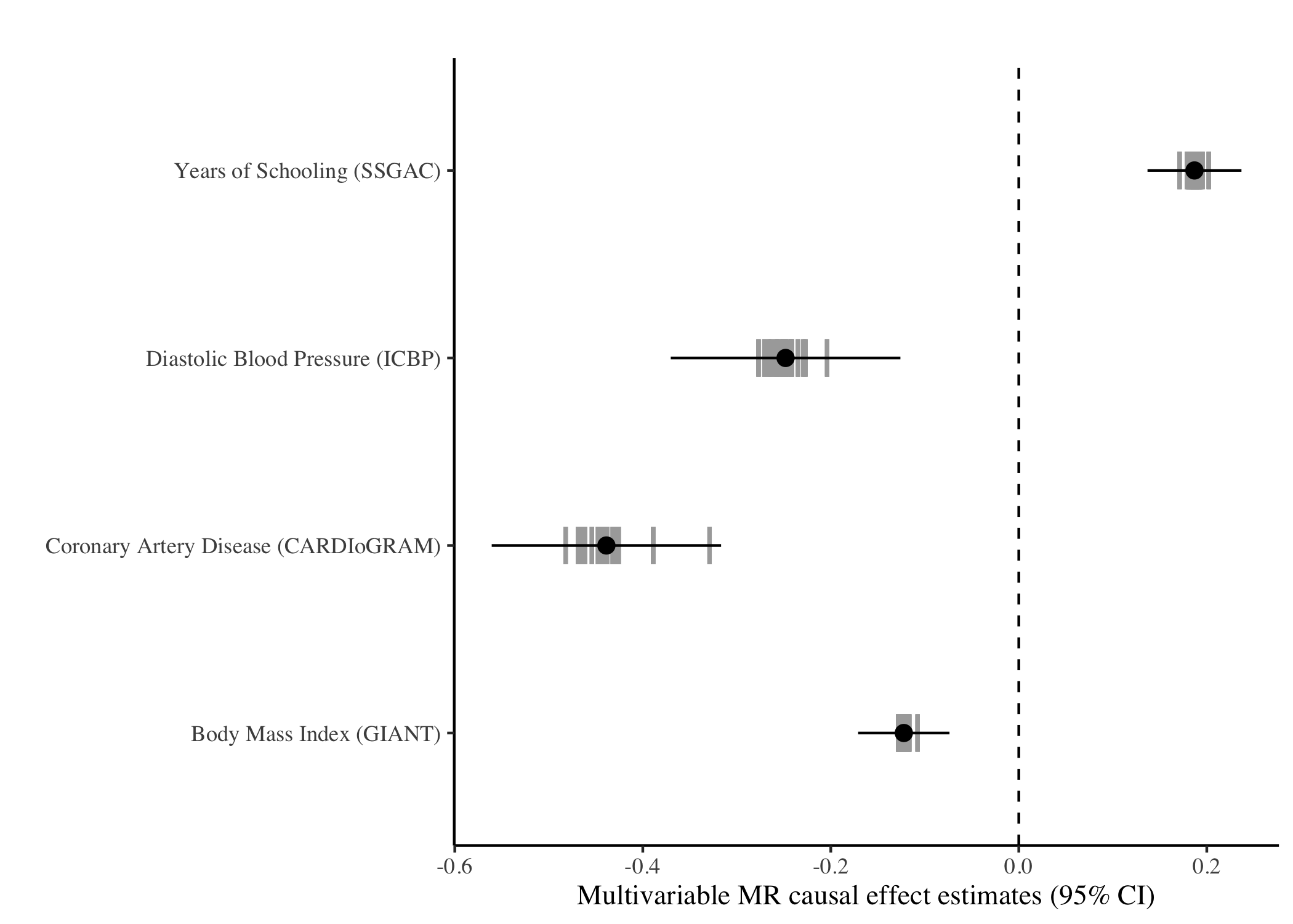
## 4 studies used to build the prior :
## # A tibble: 4 x 3
## study estimate std_error
## <chr> <dbl> <dbl>
## 1 EDUyears_2016_sumstat.txt 0.187 0.0255
## 2 All_ancestries_SNP_gwas_mc_merge_nogc.tbl.uniq.gz -0.122 0.0248
## 3 cardiogram_gwas_results.txt -0.439 0.0623
## 4 DBP -0.248 0.0623
##
## -_-_-_-_-_-_-_-_-_-_-_-_-_-_-_
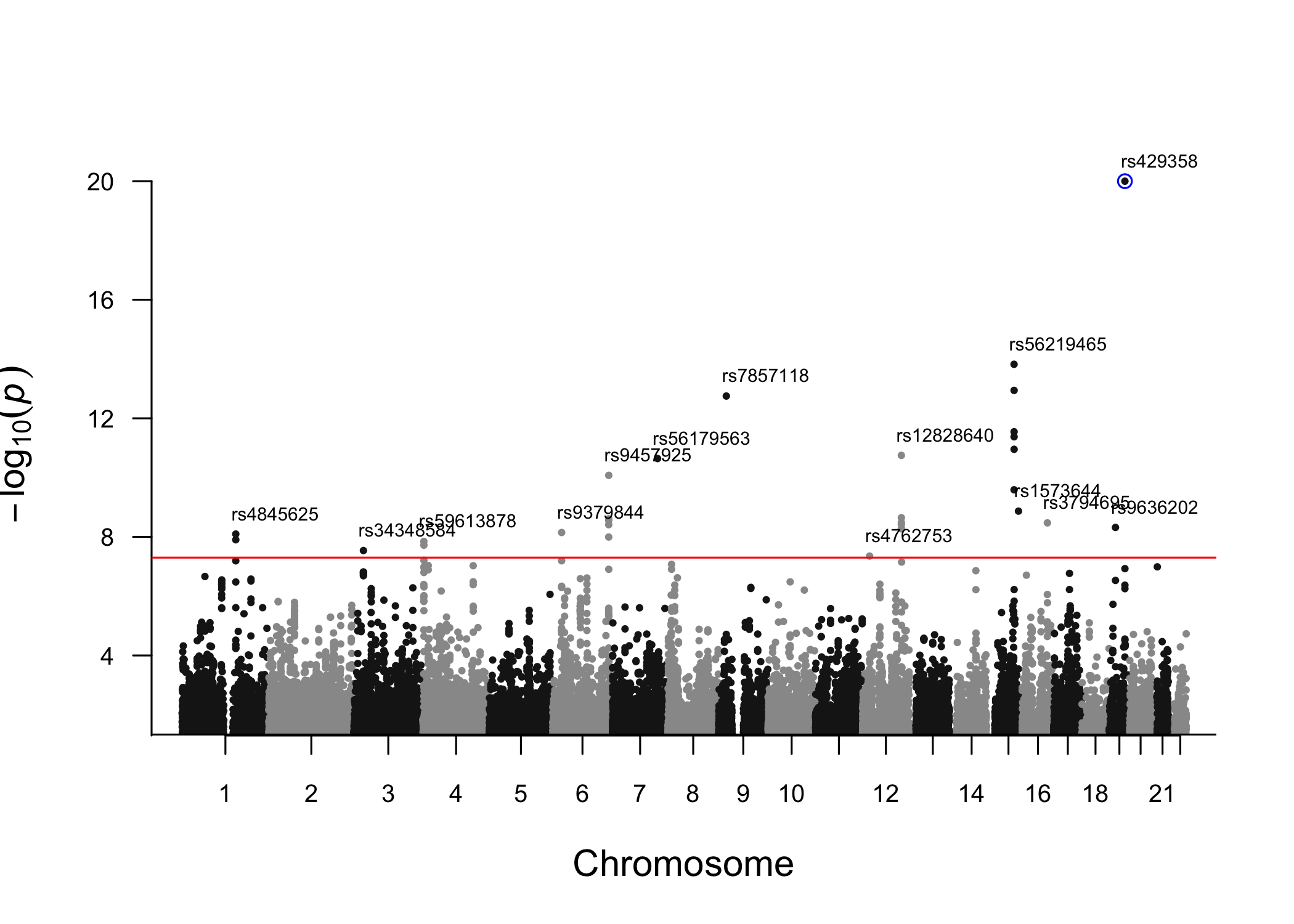
##
## 14 significant SNPs identified :
## rs429358, rs56219465, rs7857118, rs12828640, rs56179563, rs9457925, rs1573644, rs3794695, rs9636202, rs9379844, rs4845625, rs59613878, rs34348584, rs4762753
##
## -_-_-_-_-_-_-_-_-_-_-_-_-_-_-_
print_log_bGWAS(A)Show log
```
## <<< Preparation of analysis >>>
##
## > Checking parameters
## The name of your analysis is: "Test_UsingSmallDataFrame".
## The Z-Matrix files are stored in "/Users/nmounier/ZMatrices".
## # Preparation of the data...
## The conventional GWAS used as input the object: "GWAS".
##    SNPID column, ok - ALT column, ok - REF column, ok - BETA column, ok - SE column, ok
## Posterior effects will be rescaled using BETA and SE.
## The analysis will be run in the folder: "/Users/nmounier/Documents/SGG/Projects/Packaging/bGWAS".
## The p-value threshold used for selecting MR instruments is: 1e-06.
## The minimum number instruments required for each trait is: 3.
## The distance used for pruning MR instruments is: 500Kb.
## Distance-based pruning will be used for MR instruments.
## No shrinkage applied before performing MR.
## The p-value threshold used for stepwise selection is 0.05.
## Using MR_shrinkage as default for prior_shrinkage:
## No shrinkage applied before performing calculating the prior.
## The p-value threshold used for stepwise selection is 0.05.
## Significant SNPs will be identified according to p-value. The threshold used is :5e-08.
## The distance used for pruning results is: 500Kb.
## Distance-based pruning will be used for results.
##
##
## <><><><><><><><><><><><><><><><><><><><><><><><><><><><><><><><><><><><><><><><><><><><>
## <<< Identification of significant prior GWASs for MR >>>
##
## > Creating the Z-Matrix of strong instruments
## # Loading the ZMatrix...
## Selecting studies :
## 6 studies
## 209,840 SNPs
## # Adding data from the conventional GWAS :  "GWAS"
## Done!
## 8,813 SNPs in common between prior studies and the conventional GWAS
## # Thresholding...
## 767 SNPs left after thresholding
## 6 studies left after thresholding
## Pruning MR instruments...
##    distance : 500Kb
## 159 SNPs left after pruning
## 6 studies left after thresholding+pruning
##
## > Performing MR
## #Preparation of the MR analyses to identify significant studies...
## Conventionnal GWAS of interest : GWAS
## # Univariable regressions for each trait...
##   Number of trait-specific instruments per univariable regression:
##   . Body Mass Index (GIANT) : 59
##   . Coronary Artery Disease (CARDIoGRAM) : 6
##   . Years of Schooling (SSGAC) : 83
##   . Systolic Blood Pressure (ICBP) : 8
##   . Diastolic Blood Pressure (ICBP) : 8
##   . College Completion (SSGAC) : 4
## Done!
## # Stepwise selection (all traits)...
## Studies tested (reaching p<0.05 in univariable models) :  Years of Schooling (SSGAC)  Body Mass Index (GIANT)  Coronary Artery Disease (CARDIoGRAM)  Systolic Blood Pressure (ICBP)  Diastolic Blood Pressure (ICBP)
## Adding the first study :Years of Schooling (SSGAC)
## #Test if any study can be added with p<0.05
## Adding one study :Systolic Blood Pressure (ICBP)
## Done!
## #Test if any study has p>0.05 now
## #Test if any study can be added with p<0.05
## Adding one study :Body Mass Index (GIANT)
## Done!
## #Test if any study has p>0.05 now
## #Test if any study can be added with p<0.05
## Adding one study :Coronary Artery Disease (CARDIoGRAM)
## Done!
## #Test if any study has p>0.05 now
## #Test if any study can be added with p<0.05
## Adding one study :Diastolic Blood Pressure (ICBP)
## Done!
## #Test if any study has p>0.05 now
## Excluding one study :Systolic Blood Pressure (ICBP)
## Done!
## #Test if any study can be added with p<0.05
## #Test if any study has p>0.05 now
## It converged!
## # Final regression...
## The studies used are:
## - Years of Schooling (SSGAC)- Body Mass Index (GIANT)- Coronary Artery Disease (CARDIoGRAM)- Diastolic Blood Pressure (ICBP)
##
## Estimating adjusted R-squared:
## - in-sample adjusted R-squared for the all-chromosomes multivariable regression is 0.5534
## - out-of-sample R-squared (masking one chromosome at a time), for the multivariable regression will be estimated when calculating the prior.
##
##
## <><><><><><><><><><><><><><><><><><><><><><><><><><><><><><><><><><><><><><><><><><><><>
## <<< Estimation of the prior >>>
##
## > Creating the full Z-Matrix
## # Loading the ZMatrix...
## Selecting studies :
## 4 studies
## 6,811,310 SNPs
## # Adding data from the conventional GWAS :  "GWAS"
## Done!
## 286,807 SNPs in common between prior studies and the conventional GWAS
##
## > Computing prior
## # Calculating the prior chromosome by chromosome...
##    Chromosome 1
## Running regression,
## Calculating prior estimates for SNPs on this chromosome,
## Calculating prior standard errors for SNPs on this chromosome,
##    Chromosome 2
## Running regression,
## Calculating prior estimates for SNPs on this chromosome,
## Calculating prior standard errors for SNPs on this chromosome,
##    Chromosome 3
## Running regression,
## Calculating prior estimates for SNPs on this chromosome,
## Calculating prior standard errors for SNPs on this chromosome,
##    Chromosome 4
## Running regression,
## Calculating prior estimates for SNPs on this chromosome,
## Calculating prior standard errors for SNPs on this chromosome,
##    Chromosome 5
## Running regression,
## Calculating prior estimates for SNPs on this chromosome,
## Calculating prior standard errors for SNPs on this chromosome,
##    Chromosome 6
## Running regression,
## Calculating prior estimates for SNPs on this chromosome,
## Calculating prior standard errors for SNPs on this chromosome,
##    Chromosome 7
## Running regression,
## Calculating prior estimates for SNPs on this chromosome,
## Calculating prior standard errors for SNPs on this chromosome,
##    Chromosome 8
## Running regression,
## Calculating prior estimates for SNPs on this chromosome,
## Calculating prior standard errors for SNPs on this chromosome,
##    Chromosome 9
## Running regression,
## Calculating prior estimates for SNPs on this chromosome,
## Calculating prior standard errors for SNPs on this chromosome,
##    Chromosome 10
## Running regression,
## Calculating prior estimates for SNPs on this chromosome,
## Calculating prior standard errors for SNPs on this chromosome,
##    Chromosome 11
## Running regression,
## Calculating prior estimates for SNPs on this chromosome,
## Calculating prior standard errors for SNPs on this chromosome,
##    Chromosome 12
## Running regression,
## Calculating prior estimates for SNPs on this chromosome,
## Calculating prior standard errors for SNPs on this chromosome,
##    Chromosome 13
## Running regression,
## Calculating prior estimates for SNPs on this chromosome,
## Calculating prior standard errors for SNPs on this chromosome,
##    Chromosome 14
## Running regression,
## Calculating prior estimates for SNPs on this chromosome,
## Calculating prior standard errors for SNPs on this chromosome,
##    Chromosome 15
## Running regression,
## Calculating prior estimates for SNPs on this chromosome,
## Calculating prior standard errors for SNPs on this chromosome,
##    Chromosome 16
## Running regression,
## Calculating prior estimates for SNPs on this chromosome,
## Calculating prior standard errors for SNPs on this chromosome,
##    Chromosome 17
## Running regression,
## Calculating prior estimates for SNPs on this chromosome,
## Calculating prior standard errors for SNPs on this chromosome,
##    Chromosome 18
## Running regression,
## Calculating prior estimates for SNPs on this chromosome,
## Calculating prior standard errors for SNPs on this chromosome,
##    Chromosome 19
## Running regression,
## Calculating prior estimates for SNPs on this chromosome,
## Calculating prior standard errors for SNPs on this chromosome,
##    Chromosome 20
## Running regression,
## Calculating prior estimates for SNPs on this chromosome,
## Calculating prior standard errors for SNPs on this chromosome,
##    Chromosome 21
## Running regression,
## Calculating prior estimates for SNPs on this chromosome,
## Calculating prior standard errors for SNPs on this chromosome,
##    Chromosome 22
## Running regression,
## Calculating prior estimates for SNPs on this chromosome,
## Calculating prior standard errors for SNPs on this chromosome,
## ## Out-of-sample R-squared for MR instruments across all chromosomes is 0.5206
## ## Out-of-sample squared correlation for MR instruments across all chromosome is 0.5271
## ## Correlation between prior and observed effects for all SNPs is 0.1855
## ## Correlation between prior and observed effects for SNPs with GWAS p-value < 0.001 is 0.5944
## Done!
##
##
## <><><><><><><><><><><><><><><><><><><><><><><><><><><><><><><><><><><><><><><><><><><><>
## <<< Calculation of Bayes Factors and p-values >>>
##
## > Calculating them for all SNPs
## # Computing observed Bayes Factor for all SNPs...
## Done!
## # Computing BF p-values...
##    using a distribution approach:
## ... getting approximated p-values using non-linear quantiles
## ... checking p-values near significance threshold
##     everything is ok!
## # Estimating p-values for posterior effects...
## Done!
## # Estimating p-values for direct effects...
## Done!
## > Pruning and identifying significant SNPs
## Identification based on BFs
##    Starting with 286,807 SNPs
## # Selecting significant SNPs according to p-values...
## 30 SNPs left
## Done!
## # Pruning significant SNPs...
##    distance : 500Kb
## 14 SNPs left
## Done!
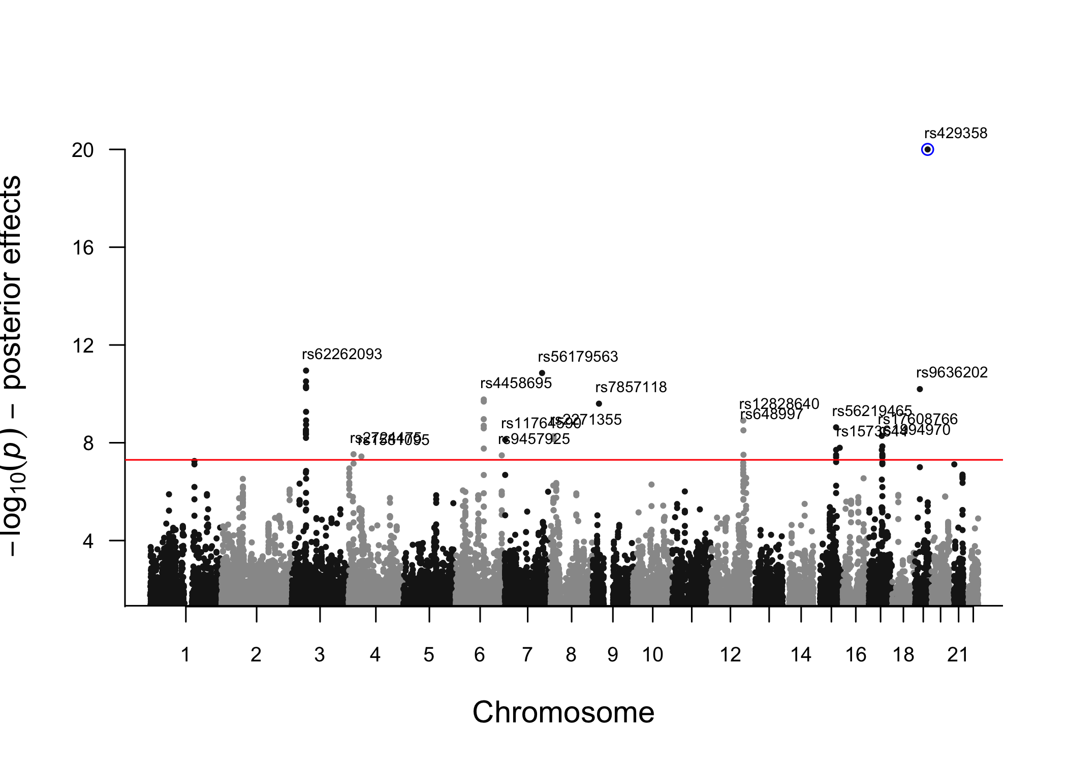
## Identification based on posterior effects
##    Starting with 286,807 SNPs
## # Selecting significant SNPs according to p-values...
## 44 SNPs left
## Done!
## # Pruning significant SNPs...
##    distance : 500Kb
## 17 SNPs left
## Done!
## Identification based on direct effects
##    Starting with 286,807 SNPs
## # Selecting significant SNPs according to p-values...
## 4 SNPs left
## Done!
## # Pruning significant SNPs...
##    distance : 500Kb
## 2 SNPs left
## Done!
##
##
## <><><><><><><><><><><><><><><><><><><><><><><><><><><><><><><><><><><><><><><><><><><><>
## Time of the analysis: 2 minute(s) and 16 second(s).
```
- Functions to extract results from an object of class bGWAS:
# by default, extract "BF" results...
hits = extract_results_bGWAS(A, SNPs = "significant")
hits
## # A tibble: 14 x 14
## rsid chrm_UK10K pos_UK10K alt ref beta se z_obs
## <chr> <dbl> <dbl> <chr> <chr> <dbl> <dbl> <dbl>
## 1 rs429358 19 45411941 T C 0.106 0.00546 19.3
## 2 rs56219465 15 78742579 A G 0.0380 0.00410 9.27
## 3 rs7857118 9 22124140 A T 0.0240 0.00387 6.20
## 4 rs12828640 12 111361298 A G -0.0229 0.00399 -5.74
## 5 rs56179563 7 129685597 A G 0.0211 0.00406 5.19
## 6 rs9457925 6 160848743 A G -0.0875 0.0145 -6.03
## 7 rs1573644 15 91421283 T C 0.0201 0.00412 4.88
## 8 rs3794695 16 72097827 T C -0.0260 0.00491 -5.30
## 9 rs9636202 19 18449238 A G 0.0194 0.00441 4.40
## 10 rs9379844 6 26291527 A G 0.0219 0.00399 5.50
## 11 rs4845625 1 154422067 T C -0.0180 0.00389 -4.63
## 12 rs59613878 4 3139152 T C 0.0206 0.00420 4.90
## 13 rs34348584 3 27532704 T C 0.0201 0.00450 4.46
## 14 rs4762753 12 20579969 T G 0.0259 0.00487 5.31
## mu_prior_estimate mu_prior_std_error beta_prior_estimate beta_prior_std_error
## <dbl> <dbl> <dbl> <dbl>
## 1 -0.351 0.611 -0.00192 0.00334
## 2 0.790 0.622 0.00324 0.00255
## 3 2.61 0.876 0.0101 0.00339
## 4 -2.34 0.680 -0.00934 0.00271
## 5 3.37 0.737 0.0137 0.00299
## 6 -1.72 0.631 -0.0250 0.00915
## 7 2.43 0.696 0.0100 0.00287
## 8 -1.69 0.608 -0.00831 0.00298
## 9 3.12 0.630 0.0137 0.00278
## 10 1.43 0.564 0.00571 0.00225
## 11 -2.29 0.665 -0.00891 0.00259
## 12 1.78 0.607 0.00750 0.00255
## 13 2.11 0.698 0.00950 0.00314
## 14 1.16 0.611 0.00564 0.00298
## BF BF_p
## <dbl> <dbl>
## 1 7.00e19 5.90e-37
## 2 2.11e 7 1.51e-14
## 3 4.32e 6 1.77e-13
## 4 2.27e 5 1.78e-11
## 5 1.95e 5 2.28e-11
## 6 8.63e 4 8.38e-11
## 7 1.60e 4 1.35e- 9
## 8 9.34e 3 3.36e- 9
## 9 7.60e 3 4.79e- 9
## 10 6.04e 3 7.12e- 9
## 11 5.64e 3 8.03e- 9
## 12 4.07e 3 1.42e- 8
## 13 2.72e 3 2.89e- 8
## 14 2.14e 3 4.43e- 8
all_results = extract_results_bGWAS(A, SNPs = "all")
nrow(all_results)
## [1] 286807
# but also possible to extract SNPs with significant posterior/direct effects
extract_results_bGWAS(A, SNPs = "significant", results = "direct")
## # A tibble: 2 x 15
## rsid chrm_UK10K pos_UK10K alt ref beta se z_obs
## <chr> <dbl> <dbl> <chr> <chr> <dbl> <dbl> <dbl>
## 1 rs429358 19 45411941 T C 0.106 0.00546 19.3
## 2 rs11633958 15 78862064 T C -0.0418 0.00410 -10.2
## mu_direct_estimate mu_direct_std_error beta_direct_estimate
## <dbl> <dbl> <dbl>
## 1 19.7 1.17 0.108
## 2 -9.99 1.18 -0.0410
## beta_direct_std_error z_direct p_direct CRR
## <dbl> <dbl> <dbl> <dbl>
## 1 0.00640 16.8 2.96e-63 1.02
## 2 0.00482 -8.50 1.90e-17 0.981
extract_MRcoeffs_bGWAS(A)[,1:12]## # A tibble: 4 x 12
## name
## <chr>
## 1 Years of Schooling (SSGAC)
## 2 Body Mass Index (GIANT)
## 3 Coronary Artery Disease (CARDIoGRAM)
## 4 Diastolic Blood Pressure (ICBP)
## study estimate std_error Tstat P chrm1_estimate chrm1_std_error
## <chr> <dbl> <dbl> <dbl> <dbl> <dbl> <dbl>
## 1 EDUyears_201… 0.187 0.0255 7.33 1.32e-11 0.187 0.0258
## 2 All_ancestri… -0.122 0.0248 -4.93 2.12e- 6 -0.108 0.0259
## 3 cardiogram_g… -0.439 0.0623 -7.05 6.18e-11 -0.469 0.0616
## 4 DBP -0.248 0.0623 -3.98 1.07e- 4 -0.264 0.0619
## chrm1_P chrm2_estimate chrm2_std_error chrm2_P
## <dbl> <dbl> <dbl> <dbl>
## 1 2.93e-11 0.186 0.0273 3.01e-10
## 2 5.55e- 5 -0.124 0.0268 8.72e- 6
## 3 4.27e-12 -0.439 0.0685 2.24e- 9
## 4 3.78e- 5 -0.250 0.0653 1.93e- 4
- Functions for graphic representations:
# Coefficients plot
coefficients_plot_bGWAS(A)
# Manhattan plot using BFs p-values
manhattan_plot_bGWAS(A)# Manhattan plot using posterior p-values
manhattan_plot_bGWAS(A, results="posterior")- .log - log file
- PriorGWASs.tsv - contains information about all prior GWASs (general info + status (used/removed) + univariable/multivariable MR estimates)
- CoefficientsByChromosome.csv - contains the multivariable MR estimates when masking the focal chromosome (22 coefficients for each prior GWASs used for prior estimation)
- PriorBFp.csv - contains BF and p-values, prior, posterior and direct effects estimates for all SNPs
- SignificantSNPs.csv - contains BF and p-values, prior, posterior and direct effects estimates for a subset of significant SNPs (identified according to specified parameters)
A detailed description of these files can be found here.
Analysis using all the 38 prior GWASs available, for a conventional GWAS containing ~7M SNPs in common with the prior studies ~ 25 minutes.
Analysis using 6 prior GWASs, for a conventional GWAS containing ~ 300,000 SNPs in common with prior studies (see example A) ~ 2 minutes.
Results from analyses performed on a MacBook Pro (Early 2015) - Processor : 2.9 GHz Intel Core i5 - Memory : 8 GB 1867 MHz DDR3.
This method has been applied to Lifespan analysis in McDaid et
al and Timmers et
al.
The most recent results (obtained using bGWAS version 1.0.2) are
available here and summarised in this
poster.
If you use the bGWAS package, please cite:


