JuliaCon 2021 workshop | Fri, July 23, 10am-1pm ET (16:00-19:00 CEST)
👀 watch the workshop LIVE recording
👉 Useful notes:
- 💡 The Getting started will help you set up.
- ❓ Further interests in solving PDEs with Julia on GPUs
- Check out this online geo-HPC tutorial
- Visit EGU21's short course repo
This workshop covers trendy areas in modern numerical computing with examples from geoscientific applications. The physical processes governing natural systems' evolution are often mathematically described as systems of differential equations or partial differential equations (PDE). Fast and accurate solutions require numerical implementations to leverage modern parallel hardware.
- Objectives
- About this repository
- Getting started (not discussed during the workshop)
- 👉 Workshop material
- Extras (optional if time permits)
- Further reading
The goal of this workshop is to offer an interactive hands-on to solve systems of differential equations in parallel on GPUs using the ParallelStencil.jl and ImplicitGlobalGrid.jl Julia packages. ParallelStencil.jl permits to write architecture-agnostic parallel high-performance GPU and CPU code for stencil computations and ImplicitGlobalGrid.jl renders its distributed parallelization almost trivial. The resulting codes are fast, short and readable [1, 2, 3].
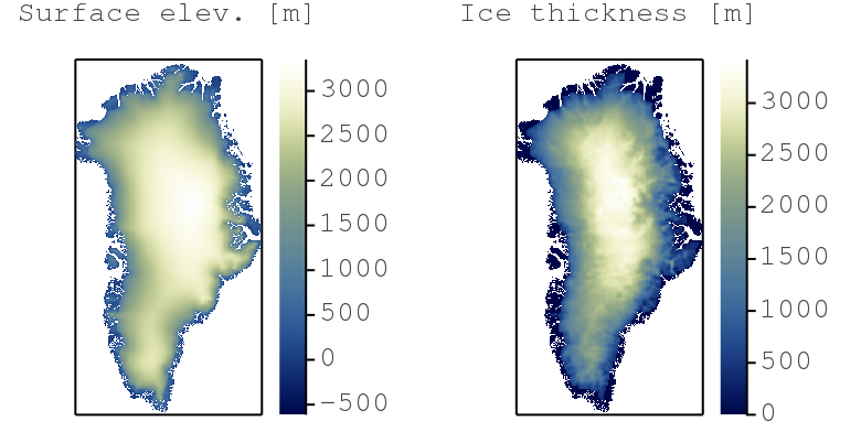
We will use these two Julia packages to design and implement an iterative nonlinear diffusion solver. We will, in a second step, turn the serial CPU solver into a parallel application to run on multiple CPU threads and on GPUs. We will, in a third step, do distributed memory computing, enhancing the nonlinear diffusion solver to execute on multiple CPUs and GPUs. The nonlinear diffusion solver we will work on can be applied to resolve the shallow ice approximation (SIA) equations with applications that predict ice flow dynamics over mountainous Greenland topography (Fig. below).
👉 Visit EGU21's short course repo if interested.
The workshop consists of 3 parts:
- Part 1 - You will learn about accelerating iterative solvers.
- Part 2 - You will port the iterative solver to parallel CPU and GPU execution.
- Part 3 - You will learn how to implement multi-CPU and multi-GPU execution.
By the end of this workshop, you will:
- Have high-performance nonlinear PDE GPU solvers;
- Have a Julia code that achieves similar performance than legacy codes (C/CUDA C + MPI);
- Be able to leverage the computing power of modern GPU accelerated servers and supercomputers.
The workshop repository lists following folders and items:
- the docs folder contains documentation linked in the README;
- the scripts folder contains the scripts this workshop is about 🎉
- the extras folder contains supporting workshop material (not discussed live during the workshop);
- the
Project.tomlfile is the Julia project file, tracking the used packages and enabling a reproducible environment.
👉 This repository is an interactive and dynamic source of information related to the workshop.
- Check out the Discussion tab if you have general comments, ideas to share or for Q&A.
- File an Issue if you encounter any technical problems with the distributed codes.
- Interact in an open-minded, respectful and inclusive manner.
TL;DR (assuming you have Julia v1.6 installed). Run at shell:
git clone https://github.com/luraess/parallel-gpu-workshop-JuliaCon21.git
cd parallel-gpu-workshop-JuliaCon21/scripts
julia --project -t4

julia> using Pkg; Pkg.instantiate()
⚠️ The workshop will not cover the Getting started steps. These are meant to provide directions to the participant willing to actively try out the examples during the workshop or for Julia newcomers. It is warmly recommended to perform the Getting started steps before the beginning of the workshop.
The detailed steps in the dropdown hereafter will get you started with:
- Installing Julia v1.6;
- Running the scripts from the workshop repository.
CLICK HERE for the getting started steps 🚀
Check you have an active internet connexion and download Julia v1.6 for your platform following the install directions provided under [help] if needed.
Alternatively, open a terminal and download the binaries (select the one for your platform):
wget https://julialang-s3.julialang.org/bin/winnt/x64/1.6/julia-1.6.1-win64.exe # Windows
wget https://julialang-s3.julialang.org/bin/mac/x64/1.6/julia-1.6.1-mac64.dmg # macOS
wget https://julialang-s3.julialang.org/bin/linux/x64/1.6/julia-1.6.1-linux-x86_64.tar.gz # Linux x86
Then add Julia to PATH (usually done in your .bashrc, .profile, or config file).
Ensure you have a text editor with syntax highlighting support for Julia. From within the terminal, type
juliato make sure that the Julia REPL (aka terminal) starts. Exit with Ctrl-d.
If you'd enjoy a more IDE type of environment, check out VS Code. Follow the installation directions for the Julia VS Code extension.
To get started with the workshop,
- clone (or download the ZIP archive) the workshop repository (help here)
git clone https://github.com/luraess/parallel-gpu-workshop-JuliaCon21.git- Navigate to
parallel-gpu-workshop-JuliaCon21
cd parallel-gpu-workshop-JuliaCon21- From the terminal, launch Julia with the
--projectflag to read-in project environment related informations such as used packages
julia --project- From VS Code, follow the instructions from the documentation to get started.
Now that you launched Julia, you should be in the Julia REPL. You need to ensure all the packages you need are installed before using them. To do so, enter the Pkg mode by typing ]. Then, instantiate the project which should trigger the download of the packages (st lists the package status). Exit the Pkg mode with Ctrl-c:
julia> ]

(parallel-gpu-workshop-JuliaCon21) pkg> st
Status `~/parallel-gpu-workshop-JuliaCon21/Project.toml`
    # [...]

(parallel-gpu-workshop-JuliaCon21) pkg> instantiate
   Updating registry at `~/.julia/registries/General`
   Updating git-repo `https://github.com/JuliaRegistries/General.git`
   # [...]

julia>
To test your install, go to the scripts folder and run the diffusion_2D_expl.jl code. You can execute shell commands from within the Julia REPL first typing ;:
julia> ;

shell> cd scripts/

julia> include("diffusion_2D_expl.jl")
Running this the first time will (pre-)complie the various installed packages and will take some time. Subsequent runs, by executing include("diffusion_2D_expl.jl"), should take around 2s.
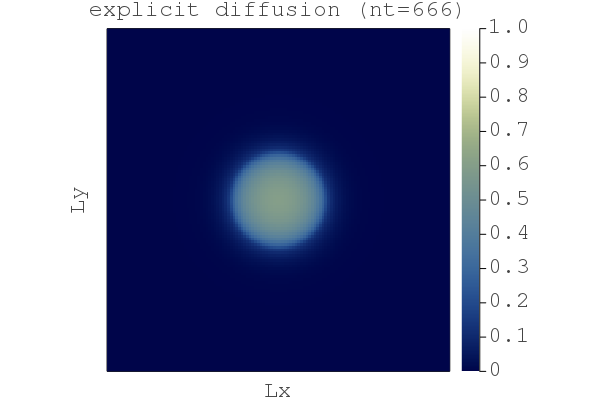
You should then see a figure displayed showing the nonlinear diffusion of a quantity H after nt=666 steps:
On the CPU, multi-threading is made accessible via Base.Threads. To make use of threads, Julia needs to be launched with
julia --project -t autowhich will launch Julia with as many threads are there are cores on your machine (including hyper-threaded cores). Alternatively set
the environment variable JULIA_NUM_THREADS, e.g. export JULIA_NUM_THREADS=2 to enable 2 threads.
The CUDA.jl module permits to launch compute kernels on Nvidia GPUs natively from within Julia. JuliaGPU provides further reading and introductory material about GPU ecosystems within Julia. If you have an Nvidia CUDA capable GPU device, also export following environment vaiable prior to installing the CUDA.jl package:
export JULIA_CUDA_USE_BINARYBUILDER=falseThe following steps permit you to install MPI.jl on your machine and test it:
-
Julia MPI being a dependency of this Julia project MPI.jl should have been added upon executing the
instantiatecommand from within the package manager see here. -
Install
mpiexecjl:
julia> using MPI

julia> MPI.install_mpiexecjl()
[ Info: Installing `mpiexecjl` to `HOME/.julia/bin`...
[ Info: Done!-
Then, one should add
HOME/.julia/binto PATH in order to launch the Julia MPI wrappermpiexecjl. -
Running a Julia MPI code
<my_script.jl>onnpprocesses:
$ mpiexecjl -n np julia --project <my_script.jl>- To test the Julia MPI installation, launch the
hello_mpi.jlusing the Julia MPI wrappermpiexecjl(located in~/.julia/bin) on 4 processes:
$ mpiexecjl -n 4 julia --project extras/hello_mpi.jl
$ Hello world, I am 0 of 3
$ Hello world, I am 1 of 3
$ Hello world, I am 2 of 3
$ Hello world, I am 3 of 3
💡 Note: On MacOS, you may encounter this issue (JuliaParallel/MPI.jl#407). To fix it, define following
ENVvariable:
$ export MPICH_INTERFACE_HOSTNAME=localhostand add
-host localhostto the execution script:
$ mpiexecjl -n 4 -host localhost julia --project extras/hello_mpi.jl👉 Note: This workshop was developed and tested on Julia v1.6. It should work with any Julia version ≥v1.6. The install configurations were tested on a MacBook Pro running macOS 10.15.7, a Linux GPU server running Ubuntu 20.04 LTS and a Linux GPU server running CentOS 8.
This section lists the material discussed within this 3h workshop:
- Part 1 - GPU computing and iterative solvers
- Part 2 - Parallel CPU and GPU computing
- Part 3 - Distributed computing on multiple CPUs and GPUs
💡 In this workshop we will implement a 2D nonlinear diffusion equation on GPUs in Julia using the finite-difference method and an iterative solving approach.
In this first part of the workshop we will implement an efficient implicit iterative and matrix-free solver to solve the time-dependent nonlinear diffusion equation in 2D.
Let's start with a 2D nonlinear diffusion example to implement both an explicit and iterative implicit PDE solver:
dH/dt = ∇.(H^3 ∇H)
The diffusion of a quantity H over time t can be described as (1a, 1b) a diffusive flux, (1c) a flux balance and (1d) an update rule:
qHx   = -H^3*dH/dx         (1a)
qHy   = -H^3*dH/dy         (1b)
dHdt  = -dqHx/dx -dqHy/dy  (1c)
dH/dt = dHdt               (1d)
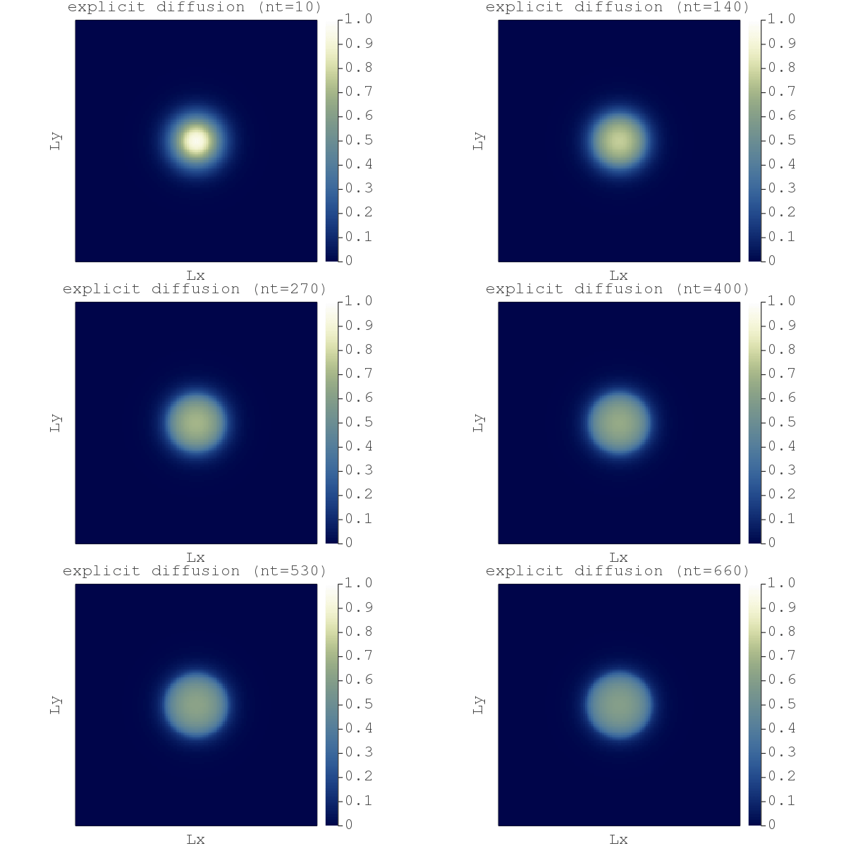
The diffusion_2D_expl.jl code implements an iterative and explicit solution of eq. (1) for an initial Gaussian profile:
H0 = exp(-(x-lx/2.0)^2 -(y-ly/2.0)^2)💡 The animation above was generated using the
diffusion_2D_expl_gif.jlscript located in extras.
A simple way to solve nonlinear diffusion, BUT:
- given the explicit nature of the scheme we have a restrictive limitation on the maximal allowed time step (subject to the CFL stability condition):
dt = minimum(min(dx, dy)^2 ./ inn(H).^npow ./ 4.1)
- there might be loss of accuracy since we use an explicit scheme for a nonlinear problem.
So now you may ask: can we use an implicit algorithm to ensure nonlinear accuracy, side-step the CFL-condition, control the (physically motivated) time steps dt and keep it "matrix-free" ?
The diffusion_2D_impl.jl code implements an iterative, implicit solution of eq. (1). How ? We include the physical time derivative dH/dt=(H-Hold)/dt in the previous rate of change dHdt to define the residual ResH
ResH = -(H-Hold)/dt -dqHx/dx -dqHy/dy = 0This is the backward Euler time-stepping scheme. We iterate until the values of ResH (the residual of the eq. (1)) drop below a defined tolerance level tol.
How do we iterate? Let's define a "new" time, a pseudo-time tau and set
dH/dtau = ResHIf we evolve H forward in pseudo-time until it reaches a steady state, we get a H which solves the equation ResH=0. This is know as a Picard or fixed-point iteration.
Running the implementation diffusion_2D_impl.jl gives:
It works, but the "naive" Picard iteration count seems to be pretty high (niter>800). A efficient way to circumvent this is to add "damping" (damp) to the (pseudo-time) rate-of-change dH/dtau, analogous to add friction enabling faster convergence [4]
dH/dtau = ResH + damp * (dH/dtau)_prevwhere (dH/dtau)_prev is the dH/dtau value from the previous pseudo-time iteration.
The diffusion_2D_damp.jl code implements a damped iterative implicit solution of eq. (1). The iteration count drops to niter<200.
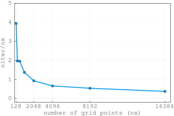
This second order pseudo-transient approach enables the iteration count to scale close to O(N) and not O(N^2), resulting in a total number of iterations niter normalised by the number of grid points nx to stay constant and even decay with increasing number of grid points nx:
The
diffusion_2D_damp_perf_gpu_iters.jlcode used for scaling test, the testing and visualisation routines can be found in extras/diffusion_2D_perf_tests.
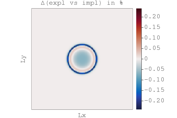
So far so good, we have a fast implicit iterative solver. But why bother with implicit, wasn't explicit good enough? Let's compare the difference between the explicit and the damped implicit results using the compare_expl_impl.jl script, chosing the "explicit" physical time step for both the explicit and implicit code:
We see that the explicit approach leads to a less sharp front by ~0.2% (when normalised by the implicit solution). (Although, arguably this 2D non-linear diffusion problem is solved similarly well by either method. But stiffer problems need an implicit time stepper.)
Efficient algorithms should minimise the time to solution. For iterative algorithms this means:
- Keep the iteration count as low as possible
- Ensure fast iterations
We just achieved (1.) with the implicit damped approach. Let's fix (2.).
Many-core processors as GPUs are throughput-oriented systems that use their massive parallelism to hide latency. On the scientific application side, most algorithms require only a few operations or flops compared to the amount of numbers or bytes accessed from main memory, and thus are significantly memory bound; the Flop/s metric is no longer the most adequate for reporting performance. This status motivated the development of a memory throughput-based performance evaluation metric, T_eff, to evaluate the performance of iterative stencil-based solvers [1].
The effective memory access, A_eff [GB], is the the sum of twice the memory footprint of the unknown fields, D_u, (fields that depend on their own history and that need to be updated every iteration, i.e. one read & one write) and once the known fields, D_k, (fields that do not change every iteration, i.e. just one read). The effective memory access divided by the execution time per iteration, t_it [sec], defines the effective memory throughput, T_eff [GB/s].
A_eff = 2 D_u + D_k
T_eff = A_eff/t_it
The theoretical upper bound of T_eff is T_peak, the hardware's peak memory throughput. Defining the T_eff metric, we assume that 1) we evaluate an iterative stencil-based solver, 2) the problem size is much larger than the cache sizes and 3) we do not use time blocking (reasonable assumption for real-world applications). An important concept is not to include fields within the effective memory access that do not depend on their own history (e.g. fluxes); such fields can be re-computed on the fly or stored on-chip.
Fore more details, check out the performance related section from ParallelStencil.jl.
For the 2D time-dependent diffusion equation, we thus have D_u=2 and D_k=1:
A_eff = (2 x 2 + 2 x 1) x 8 x nx x ny / 1e9 [GB]Let's implement this measure in the following scripts.
In this second part of the workshop, we will port the diffusion_2D_damp.jl script implemented using Julia CPU array broadcasting to high-performance parallel CPU and GPU implementations.
# [...] skipped lines
qHx    .= .-av_xi(H).^npow.*diff(H[:,2:end-1], dims=1)/dx  # flux
qHy    .= .-av_yi(H).^npow.*diff(H[2:end-1,:], dims=2)/dy  # flux
ResH   .= .-(inn(H) .- inn(Hold))/dt .+
           (.-diff(qHx, dims=1)/dx .-diff(qHy, dims=2)/dy) # residual of the PDE
dHdtau .= ResH .+ damp*dHdtau                              # damped rate of change
dtau   .= (1.0./(min(dx, dy)^2. /inn(H).^npow./4.1) .+ 1.0/dt).^-1  # time step (obeys ~CFL condition)
H[2:end-1,2:end-1] .= inn(H) .+ dtau.*dHdtau               # update rule, sets the BC as H[1]=H[end]=0
# [...] skipped lines
In the first step towards this goal we:
- use single-line broadcasting statements to avoid having to use work-arrays (to make it prettier & shorter we use macros)
- introduce a
H2array to avoid race conditions (once parallelized) - use non-allocating
diffoperators:LazyArrays: Diff - add accurate timing of the main loop and
T_effreporting
This results in the diffusion_2D_damp_perf.jl code:
using LazyArrays
using LazyArrays: Diff
# [...] skipped lines
macro qHx()  esc(:( .-av_xi(H).^npow.*Diff(H[:,2:end-1], dims=1)/dx )) end
macro qHy()  esc(:( .-av_yi(H).^npow.*Diff(H[2:end-1,:], dims=2)/dy )) end
macro dtau() esc(:( (1.0./(min(dx, dy)^2 ./inn(H).^npow./4.1) .+ 1.0/dt).^-1  )) end
# [...] skipped lines
if (it==1 && iter==0) t_tic = Base.time(); niter = 0 end
dHdtau .= .-(inn(H) .- inn(Hold))/dt .+
           (.-Diff(@qHx(), dims=1)/dx .-Diff(@qHy(), dims=2)/dy) .+
           damp*dHdtau                              # damped rate of change
H2[2:end-1,2:end-1] .= inn(H) .+ @dtau().*dHdtau    # update rule, sets the BC as H[1]=H[end]=0
H, H2 = H2, H                                       # pointer swap
# [...] skipped lines
t_toc = Base.time() - t_tic
A_eff = (2*2+1)/1e9*nx*ny*sizeof(Float64)  # Effective main memory access per iteration [GB]
t_it  = t_toc/niter                        # Execution time per iteration [s]
T_eff = A_eff/t_it                         # Effective memory throughput [GB/s]
# [...] skipped lines
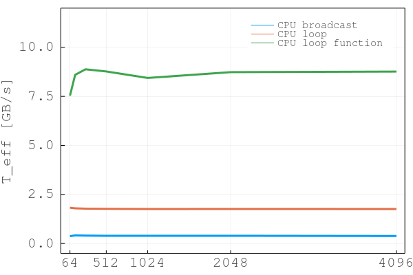
Running diffusion_2D_damp_perf.jl with nx = ny = 512, starting Julia with -O3 --check-bounds=no produces following output on an Intel Quad-Core i5-4460 CPU @3.20GHz processor (T_peak = 17 GB/s measured with memcopy3D.jl):
Time = 21.523 sec, T_eff = 0.39 GB/s (niter = 804)The next step step is to modify the diffusion code diffusion_2D_damp_perf.jl by transforming the isolated physics calculations (see end of previous section) into spatial loops over ix and iy, resulting in the diffusion_2D_damp_perf_loop.jl code:
# [...] skipped lines
macro qHx(ix,iy)  esc(:( -(0.5*(H[$ix,$iy+1]+H[$ix+1,$iy+1]))^npow * (H[$ix+1,$iy+1]-H[$ix,$iy+1])/dx )) end
macro qHy(ix,iy)  esc(:( -(0.5*(H[$ix+1,$iy]+H[$ix+1,$iy+1]))^npow * (H[$ix+1,$iy+1]-H[$ix+1,$iy])/dy )) end
macro dtau(ix,iy) esc(:(  (1.0/(min(dx,dy)^2 / H[$ix+1,$iy+1]^npow/4.1) + 1.0/dt)^-1  )) end
# [...] skipped lines
for iy=1:size(dHdtau,2)
    for ix=1:size(dHdtau,1)
        dHdtau[ix,iy] = -(H[ix+1, iy+1] - Hold[ix+1, iy+1])/dt +
                         (-(@qHx(ix+1,iy)-@qHx(ix,iy))/dx -(@qHy(ix,iy+1)-@qHy(ix,iy))/dy) +
                         damp*dHdtau[ix,iy]                        # damped rate of change
        H2[ix+1,iy+1] = H[ix+1,iy+1] + @dtau(ix,iy)*dHdtau[ix,iy]  # update rule, sets the BC as H[1]=H[end]=0
    end
end
H, H2 = H2, H  # pointer swap
# [...] skipped lines
💡 Note that macros can now take
ixandiyas arguments and that both calculations fordHdtauandHupdate are done within a single loop (loop fusion).
Running diffusion_2D_damp_perf_loop.jl with nx = ny = 512 produces following output:
Time = 4.774 sec, T_eff = 1.80 GB/s (niter = 804)(We're not sure why the performance so drastically improved over diffusion_2D_damp_perf.jl, as broadcasting was just replaced by loops.)
The next step is to wrap these physics calculations into functions (later called kernels on the GPU) and define them before the main function of the script, resulting in the diffusion_2D_damp_perf_loop_fun.jl code:
# [...] skipped lines
macro qHx(ix,iy)  esc(:( -(0.5*(H[$ix,$iy+1]+H[$ix+1,$iy+1]))*(0.5*(H[$ix,$iy+1]+H[$ix+1,$iy+1]))*(0.5*(H[$ix,$iy+1]+H[$ix+1,$iy+1])) * (H[$ix+1,$iy+1]-H[$ix,$iy+1])*_dx )) end
macro qHy(ix,iy)  esc(:( -(0.5*(H[$ix+1,$iy]+H[$ix+1,$iy+1]))*(0.5*(H[$ix+1,$iy]+H[$ix+1,$iy+1]))*(0.5*(H[$ix+1,$iy]+H[$ix+1,$iy+1])) * (H[$ix+1,$iy+1]-H[$ix+1,$iy])*_dy )) end
macro dtau(ix,iy) esc(:(  (1.0/(min_dxy2 / (H[$ix+1,$iy+1]*H[$ix+1,$iy+1]*H[$ix+1,$iy+1]) / 4.1) + _dt)^-1  )) end

function compute_update!(H2, dHdtau, H, Hold, _dt, damp, min_dxy2, _dx, _dy)
    Threads.@threads for iy=1:size(dHdtau,2)
    # for iy=1:size(dHdtau,2)
        for ix=1:size(dHdtau,1)
            dHdtau[ix,iy] = -(H[ix+1, iy+1] - Hold[ix+1, iy+1])*_dt +
                             (-(@qHx(ix+1,iy)-@qHx(ix,iy))*_dx -(@qHy(ix,iy+1)-@qHy(ix,iy))*_dy) +
                             damp*dHdtau[ix,iy]                        # damped rate of change
            H2[ix+1,iy+1] = H[ix+1,iy+1] + @dtau(ix,iy)*dHdtau[ix,iy]  # update rule, sets the BC as H[1]=H[end]=0
        end
    end
    return
end
# [...] skipped lines
_dx, _dy, _dt = 1.0/dx, 1.0/dy, 1.0/dt
min_dxy2 = min(dx,dy)^2
compute_update!(H2, dHdtau, H, Hold, _dt, damp, min_dxy2, _dx, _dy)
# [...] skipped lines
💡 Note that the outer loop (over
iy) can be parallelized using multi-threading capabilities of the CPU accessible viaThreads.@threads(see Getting started for more infos).
Running diffusion_2D_damp_perf_loop_fun.jl with nx = ny = 512 on 4 cores produces following output:
Time = 0.961 sec, T_eff = 8.80 GB/s (niter = 804)(Here again: some performance improvement stems from using multi-threading but there are additional gains compared to diffusion_2D_damp_perf_loop.jl of unknown origin...)
Since the performance increases and gets closer to hardware limit (memory copy values), some details start to become performance limiters, namely:
- divisions instead of multiplications
- arithmetic operations such as power
H^npow
These details will become even more important on the GPU.
We are now ready to move to the GPU !
So we now have a cool iterative and implicit nonlinear diffusion solver in less than 100 lines of code 🎉. Good enough for mid-resolution calculations. What if we need higher resolution and faster time to solution ? GPU computing makes it possible to go way beyond the so far achieved T_eff of 8.8 GB/s with my consumer electronics CPU. Let's slightly modify the diffusion_2D_damp_perf_loop_fun.jl code to enable GPU execution.
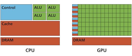
The main idea of the applied GPU parallelisation is to calculate each grid point concurrently by a different GPU thread (instead of the more serial CPU execution) as depicted hereafter:
The main change is to replace the (multi-threaded) loops by a vectorised GPU index:
ix = (blockIdx().x-1) * blockDim().x + threadIdx().x
iy = (blockIdx().y-1) * blockDim().y + threadIdx().y
specific to GPU execution. Each ix and iy are then executed concurrently by a different GPU thread. Also, whether a grid point has to participate in the calculation or not can no longer be defined by the loop range, but needs to be handled locally to each thread by e.g. an if-condition, resulting in the following diffusion_2D_damp_perf_gpu.jl GPU code:
using CUDA
# [...] skipped lines
function compute_update!(H2, dHdtau, H, Hold, _dt, damp, min_dxy2, _dx, _dy)
    ix = (blockIdx().x-1) * blockDim().x + threadIdx().x
    iy = (blockIdx().y-1) * blockDim().y + threadIdx().y
    if (ix<=size(dHdtau,1) && iy<=size(dHdtau,2))
        dHdtau[ix,iy] = -(H[ix+1, iy+1] - Hold[ix+1, iy+1])*_dt +
                         (-(@qHx(ix+1,iy)-@qHx(ix,iy))*_dx -(@qHy(ix,iy+1)-@qHy(ix,iy))*_dy) +
                         damp*dHdtau[ix,iy]                        # damped rate of change
        H2[ix+1,iy+1] = H[ix+1,iy+1] + @dtau(ix,iy)*dHdtau[ix,iy]  # update rule, sets the BC as H[1]=H[end]=0
    end
    return
end
# [...] skipped lines
BLOCKX = 32
BLOCKY = 8
GRIDX  = 16*16
GRIDY  = 32*32
nx, ny = BLOCKX*GRIDX, BLOCKY*GRIDY # number of grid points
# [...] skipped lines
ResH   = CUDA.zeros(Float64, nx-2, ny-2) # normal grid, without boundary points
dHdtau = CUDA.zeros(Float64, nx-2, ny-2) # normal grid, without boundary points
# [...] skipped lines
H      = CuArray(exp.(.-(xc.-lx/2).^2 .-(yc.-ly/2)'.^2))
# [...] skipped lines
cuthreads = (BLOCKX, BLOCKY, 1)
cublocks  = (GRIDX,  GRIDY,  1)
# [...] skipped lines
@cuda blocks=cublocks threads=cuthreads compute_update!(H2, dHdtau, H, Hold, _dt, damp, min_dxy2, _dx, _dy)
synchronize()
# [...] skipped lines
💡 We use
@cuda blocks=cublocks threads=cuthreadsto launch the GPU kernel on the appropriate number of threads, i.e. "parallel workers". The number of grid pointsnxandnymust now be chosen according to the number of parallel workers. Also, note that we need to run higher resolution in order to saturate the GPU memory bandwidth and get relevant performance measures.
⚠ Default precision in
CUDA.jlisFloat32, so we have to enforceFloat64here.
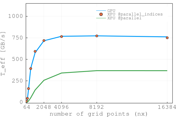
Running diffusion_2D_damp_perf_gpu.jl with nx = ny = 8192 produces the following output on an Nvidia Tesla V100 PCIe (16GB) GPU (T_peak = 840 GB/s measured with memcopy3D.jl):
Time = 10.088 sec, T_eff = 770.00 GB/s (niter = 2904)So - that rocks 🚀
Let's do a rapid recap:
So far we have two performant codes, one CPU-based, the other GPU-based, to solve the nonlinear and implicit diffusion equation in 2D. Wouldn't it be great to have a single code that enables both ?
The answer is ParallelStencil.jl which enables a backend independent syntax implementing parallel stencil kernels to execute on XPUs. The diffusion_2D_damp_perf_xpu2.jl code uses ParallelStencil.jl to combine diffusion_2D_damp_perf_gpu.jl and diffusion_2D_damp_perf_loop_fun.jl into a single code. Backend can be chosen by the USE_GPU flag. Using the parallel_indices permits to write code that avoids storing the fluxes to main memory:
const USE_GPU = true
using ParallelStencil
using ParallelStencil.FiniteDifferences2D
@static if USE_GPU
    @init_parallel_stencil(CUDA, Float64, 2)
else
    @init_parallel_stencil(Threads, Float64, 2)
end
# [...] skipped lines
@parallel_indices (ix,iy) function compute_update!(H2, dHdtau, H, Hold, _dt, damp, min_dxy2, _dx, _dy)
    if (ix<=size(dHdtau,1) && iy<=size(dHdtau,2))
        dHdtau[ix,iy] = -(H[ix+1, iy+1] - Hold[ix+1, iy+1])*_dt +
                         (-(@qHx(ix+1,iy)-@qHx(ix,iy))*_dx -(@qHy(ix,iy+1)-@qHy(ix,iy))*_dy) +
                         damp*dHdtau[ix,iy]                        # damped rate of change
        H2[ix+1,iy+1] = H[ix+1,iy+1] + @dtau(ix,iy)*dHdtau[ix,iy]  # update rule, sets the BC implicitly as H[1]=H[end]=0
    end
    return
end
# [...] skipped lines
@parallel cublocks cuthreads compute_update!(H2, dHdtau, H, Hold, _dt, damp, min_dxy2, _dx, _dy)
# [...] skipped lines
💡 Note that ParallelStencil.jl currently supports
Threads.@threadsandCUDA.jlas backends.
Running diffusion_2D_damp_perf_xpu2.jl with nx = ny = 8192 on an Nvidia Tesla V100 PCIe (16GB) GPU produces following output:
Time = 10.094 sec, T_eff = 770.00 GB/s (niter = 2904)That's excellent ! ParallelStencil.jl and the CUDA.jl backend show identical performance compared to the pure CUDA diffusion_2D_damp_perf_gpu.jl code. The diffusion_2D_damp_perf_xpu2.jl XPU code uses manually precomputed optimal grid and thread block sizes passed to the @parallel launch macro (type ?@parallel for more information). Alternatively, ParallelStencil provides some "comfort features" for launching kernels, as e.g. computing automatically and dynamically optimal grid and thread block sizes, resulting currently in about 1% performance difference (see diffusion_2D_damp_perf_gpu.jl; note that in the next release of ParallelStencil this performance difference will become entirely negligible). The "default" implementation using ParallelStencil would allow for using macros exposed by the FiniteDifferences2D module for a math-close notation in the kernels:
# [...] skipped lines
@parallel function compute_flux!(qHx, qHy, H, _dx, _dy)
    @all(qHx) = -@av_xi(H)*@av_xi(H)*@av_xi(H)*@d_xi(H)*_dx
    @all(qHy) = -@av_yi(H)*@av_yi(H)*@av_yi(H)*@d_yi(H)*_dy
    return
end

macro dtau() esc(:( (1.0/(min_dxy2 / (@inn(H)*@inn(H)*@inn(H)) / 4.1) + _dt)^-1 )) end
@parallel function compute_update!(dHdtau, H, Hold, qHx, qHy, _dt, damp, min_dxy2, _dx, _dy)
    @all(dHdtau) = -(@inn(H) - @inn(Hold))*_dt - @d_xa(qHx)*_dx - @d_ya(qHy)*_dy + damp*@all(dHdtau)
    @inn(H)      =   @inn(H) + @dtau()*@all(dHdtau)
    return
end
Running diffusion_2D_damp_xpu.jl with nx = ny = 8192 on an Nvidia Tesla V100 PCIe (16GB) GPU produces following output:
Time = 21.420 sec, T_eff = 360.00 GB/s (niter = 2904)The performance is significantly less good in this case as writing fluxes to main memory could not be avoided using the more comfortable syntax. Note, however, that in many applications we do not face this issue and the performance of applications written using the @parallel macro is on par with those written using the @parallel_indices macro.
💡 Future versions of ParallelStencil will enable comfortable syntax using the
@parallelmacro for computing fields as these fluxes on-the-fly or for storing them on-chip.
We have developed 6 scripts, 3 CPU-based and 4 GPU-based, we can now use to realise a scaling test and report T_eff as function of number of grid points nx = [64 128, 256, 512, 1024, 2048, 4096] and including [..., 8192, 16384] values on the GPU:
Note that T_peak of the Nvidia Tesla V100 GPU is 840 GB/s. Our GPU code thus achieves an effective memory throughput which is 92% of the peak memory throughput. The codes used for performance tests and testing routine can be found in extras/diffusion_2D_perf_tests.
In this last part of the workshop, we will explore multi-XPU capabilities. This will enable our codes to run on multiple CPUs and GPUs in order to scale on modern multi-GPU nodes, clusters and supercomputers. Also, we will experiment with basic concepts of the distributed memory computing approach using Julia's MPI wrapper MPI.jl. In the proposed approach, each MPI process handles one CPU thread. In the MPI GPU case (multi-GPUs), each MPI process handles one GPU. The Getting started section contains useful information in the Julia MPI section to get you set up.
As a first step, we will look at the diffusion_1D_2procs.jl code that solves the linear diffusion equations using a "fake-parallelisation" approach. We split the calculation on two distinct left and right domains, which requires left and right H arrays, HL and HR, respectively:
# Compute physics locally
HL[2:end-1] .= HL[2:end-1] .+ dt*λ*diff(diff(HL)/dx)/dx
HR[2:end-1] .= HR[2:end-1] .+ dt*λ*diff(diff(HR)/dx)/dx
# Update boundaries (later MPI)
HL[end] = HR[2]
HR[1]   = HL[end-1]
# Global picture
H .= [HL[1:end-1]; HR[2:end]]
We see that a correct boundary update is the critical part for a successful implementation. In our approach, we need an overlap of 2 cells in order to avoid any artefacts at the transition between the left and right domains.
The next step would be to generalise the "2 processes" concept to "n-processes", keeping the "fake-parallelisation" approach. The diffusion_1D_nprocs.jl code contains this modification:
for ip = 1:np # compute physics locally
    H[2:end-1,ip] .= H[2:end-1,ip] .+ dt*λ*diff(diff(H[:,ip])/dxg)/dxg
end
for ip = 1:np-1 # update boundaries
    H[end,ip  ] = H[    2,ip+1]
    H[  1,ip+1] = H[end-1,ip  ]
end
for ip = 1:np # global picture
    i1 = 1 + (ip-1)*(nx-2)
    Hg[i1:i1+nx-2] .= H[1:end-1,ip]
end
The array H contains now n local domains where each domain belongs to one fake process, namely the fake process indicated by the second index of H (ip). The # update boundaries steps are adapted accordingly. All the physical calculations happen on the local chunks of the arrays. We only need "global" knowledge in the definition of the initial condition, in order to e.g. initialise the Gaussian distribution using global and not local coordinates.
So far, so good, we are now ready to write a script that would truly distribute calculations on different processors using MPI.jl.
As next step, let's see what are the minimal requirements that would allow us to write an MPI-parallel code in Julia. We will solve the following linear diffusion physics:
for it = 1:nt
    qHx        .= .-λ*diff(H)/dx
    H[2:end-1] .= H[2:end-1] .- dt*diff(qHx)/dx
end
on multiple processors. The diffusion_1D_mpi.jl code implements the following steps:
- Initialise MPI and set-up a Cartesian communicator
- Implement a boundary exchange routine
- Finalise MPI
- Create a "global" initial condition
To (1.) initialise MPI and prepare the Cartesian communicator, we define:
MPI.Init()
dims        = [0]
comm        = MPI.COMM_WORLD
nprocs      = MPI.Comm_size(comm)
MPI.Dims_create!(nprocs, dims)
comm_cart   = MPI.Cart_create(comm, dims, [0], 1)
me          = MPI.Comm_rank(comm_cart)
coords      = MPI.Cart_coords(comm_cart)
neighbors_x = MPI.Cart_shift(comm_cart, 0, 1)
where me represents the process ID unique to each MPI process.
Then, we need to (2.) implement a boundary exchange routine. For conciseness, we will here use blocking messages:
@views function update_halo(A, neighbors_x, comm)
    if neighbors_x[1] != MPI.MPI_PROC_NULL
        sendbuf = A[2]
        recvbuf = zeros(1)
        MPI.Send(sendbuf,  neighbors_x[1], 0, comm)
        MPI.Recv!(recvbuf, neighbors_x[1], 1, comm)
        A[1] = recvbuf[1]
    end
    if neighbors_x[2] != MPI.MPI_PROC_NULL
        sendbuf = A[end-1]
        recvbuf = zeros(1)
        MPI.Send(sendbuf,  neighbors_x[2], 1, comm)
        MPI.Recv!(recvbuf, neighbors_x[2], 0, comm)
        A[end] = recvbuf[1]
    end
    return
end
In a nutshell, we store the boundary values we want to exchange in a send buffer sendbuf and initialise a receive buffer recvbuf; then, we send the content of sendbuf to the neighbor (sending messages MPI.Send(), MPI.Recv!()); finally, we assign to the boundary the values from the receive buffer.
Last, we need to (3.) finalise MPI prior to returning from the main
MPI.Finalize()The remaining step is to (4.) create an initial Gaussian distribution of H that spans correctly over all local domains. This can be achieved as following:
x0    = coords[1]*(nx-2)*dx
xc    = [x0 + ix*dx - dx/2 - 0.5*lx  for ix=1:nx]
H     = exp.(.-xc.^2)
where x0 represents the first global x-coordinate on every process and xc represents the local chunk of the global coordinates on each local process.
Running the diffusion_1D_mpi.jl code
mpiexecjl -n 4 julia --project diffusion_1D_mpi.jlwill generate one output file for each MPI process. Use the vizme1D_mpi.jl script to reconstruct the global H array from the local results and visualise it.
Yay 🎉 - we just made a Julia parallel MPI diffusion solver in only 70 lines of code.
Hold-on, the diffusion_2D_mpi.jl code implements a 2D version of the diffusion_1D_mpi.jl code. Nothing is really new there, but it may be interesting to see how boundary update routines are defined in 2D as one now needs to exchange vectors instead of single values. Running the diffusion_2D_mpi.jl will generate one output file per MPI process and the vizme2D_mpi.jl script can then be used for visualisation purpose.
Note: The presented concise Julia MPI scripts are inspired from this 2D python script.
Let's do a quick recap: so far, we explored the concept of distributed memory parallelisation with simple "fake-parallel" codes. We then demystified the usage of MPI in Julia within a 1D and 2D diffusion solver using MPI.jl, a Cartesian topology and blocking message. This code would already execute on many processors and could be launched on a cluster.
The remaining steps are to:
- use non-blocking communication
- use multiple GPUs
- prevent MPI communication to become the performance killer
We address these steps using ImplicitGlobalGrid.jl along with ParallelStencil.jl. As final act of this workshop we will take the high-performance XPU diffusion_2D_damp_perf_xpu.jl code from Part 2:
# [...] skipped lines
damp   = 1-35/nx      # damping (this is a tuning parameter, dependent on e.g. grid resolution)
dx, dy = lx/nx, ly/ny # grid size
# [...] skipped lines
H      = Data.Array(exp.(.-(xc.-lx/2).^2 .-(yc.-ly/2)'.^2))
# [...] skipped lines
@parallel compute_update!(H2, dHdtau, H, Hold, _dt, damp, min_dxy2, _dx, _dy)
# [...] skipped lines
err = norm(ResH)/length(ResH)
# [...] skipped lines
and add the few required ImplicitGlobalGrid.jl functions in order to have a multi-XPU code ready to scale on GPU supercomputers.
Appreciate the few minor changes -10 new lines only- (not including those for visualisation) required turn the single-XPU code into a multi-XPU code diffusion_2D_damp_perf_multixpu.jl:
# [...] skipped lines
using ImplicitGlobalGrid, Plots, Printf, LinearAlgebra
import MPI
# [...] skipped lines
norm_g(A) = (sum2_l = sum(A.^2); sqrt(MPI.Allreduce(sum2_l, MPI.SUM, MPI.COMM_WORLD)))
# [...] skipped lines
me, dims = init_global_grid(nx, ny, 1)  # Initialization of MPI and more...
@static if USE_GPU select_device() end  # select one GPU per MPI local rank (if >1 GPU per node)
dx, dy = lx/nx_g(), ly/ny_g()           # grid size
damp   = 1-35/nx_g()                    # damping (this is a tuning parameter, dependent on e.g. grid resolution)
# [...] skipped lines
H     .= Data.Array([exp(-(x_g(ix,dx,H)+dx/2 -lx/2)^2 -(y_g(iy,dy,H)+dy/2 -ly/2)^2) for ix=1:size(H,1), iy=1:size(H,2)])
# [...] skipped lines
len_ResH_g = ((nx-2-2)*dims[1]+2)*((ny-2-2)*dims[2]+2)
# [...] skipped lines
@hide_communication (8, 4) begin # communication/computation overlap
    @parallel compute_update!(H2, dHdtau, H, Hold, _dt, damp, min_dxy2, _dx, _dy)
    H, H2 = H2, H
    update_halo!(H)
end
# [...] skipped lines
err = norm_g(ResH)/len_ResH_g
# [...] skipped lines
finalize_global_grid()
# [...] skipped lines
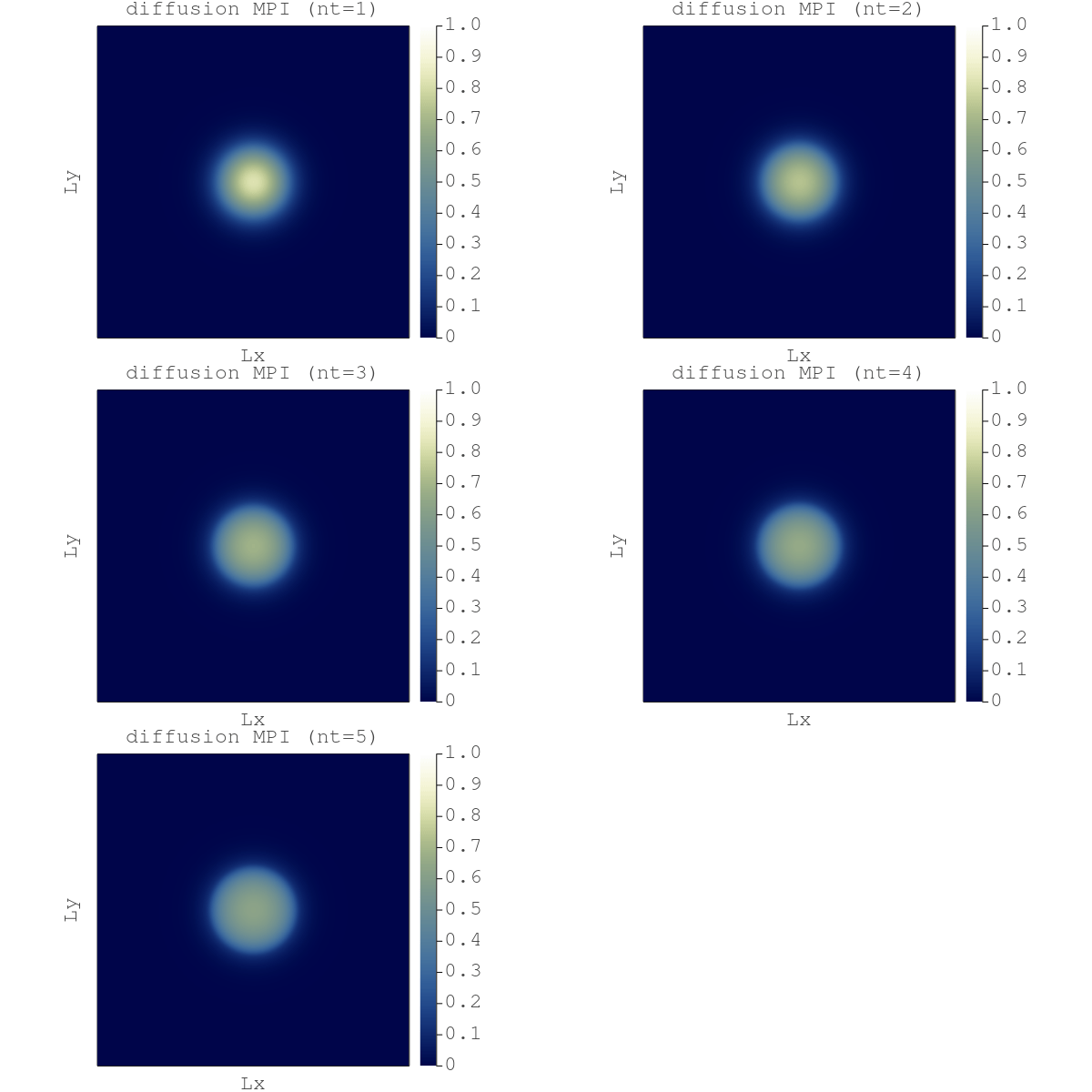
Running the diffusion_2D_damp_perf_multixpu.jl code with do_visu = true generates the following gif (here 4096x4096 grid points on 4 GPUs)
So, here we are:
We have a Julia GPU MPI code to resolve nonlinear diffusion processes in 2D using a second order accelerated iterative scheme and we can run it on GPU supercomputers 🎉.
This last section provides directions and details on more advanced features.
ImplicitGlobalGrid.jl supports CUDA-aware MPI upon exporting the ENV variable IGG_CUDAAWARE_MPI=1; MPI can then access device (GPU) pointers and exchange data directly between GPUs using Remote Direct Memory Access (RDMA) bypassing extra buffer copies to the CPU for enhanced performance.
ParallelStencil.jl exposes a hiding communication feature accessible through the @hide_communication macro. This macro allows to define a boundary width applied to each local domain in order to split the computation such that:
- The boundary cells are first computed
- The communication (boundary exchange procedure) can start
- The remaining inner points are computed while boundary exchange is on-going.
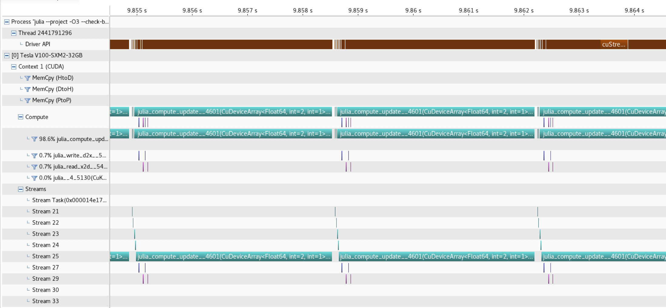
The diffusion_2D_damp_perf_multixpu_prof.jl code implements CUDA profiling features to visualise the MPI communication overlapping with computation, adding CUDA.@profile while err>tol && iter<itMax to the inner loop.
Running the code as:
mpirun -np 4 nvprof --profile-from-start off --export-profile diffusion_2D.%q{OMPI_COMM_WORLD_RANK}.prof -f julia --project -O3 --check-bounds=no diffusion_2D_damp_perf_multixpu_prof.jlwith will generate profiler files that can then be loaded and visualised Nvidia's visual profiler (nvvp):
Note that CUDA-aware MPI was used on 4 Nvidia Tesla V100 GPUs, connected with NVLink (i.e. MPI communication is using NVLink here)
The MPI communication (purple bars) nicely overlap the compute_update!() kernel execution. Further infos can be found here.
The approach and tools presented in this workshop are not restricted to 2D calculation. If you have interests in 3D examples, check out the miniapps section from the ParallelStencil.jl README. The miniapps section provides also additional information:
- about the
T_effmetric; - on how to run MPI GPU applications on different hardware.
