lvcheng1229/geometry-processing-smoothing

Smoothing assignment for Geometry Processing course

Geometry Processing – Smoothing

To get started: Fork this repository then issue

git clone --recursive http://github.com/[username]/geometry-processing-smoothing.git

Installation, Layout, and Compilation

See introduction.

Execution

Once built, you can execute the assignment from inside the build/ by running on a given mesh with given scalar field (in dmat format).

./smoothing [path to mesh.obj] [path to data.dmat]

or to load a mesh with phony noisy data use:

./smoothing [path to mesh.obj] n

or to load a mesh with smooth z-values as data (for mesh smoothing only):

./smoothing [path to mesh.obj]

Background

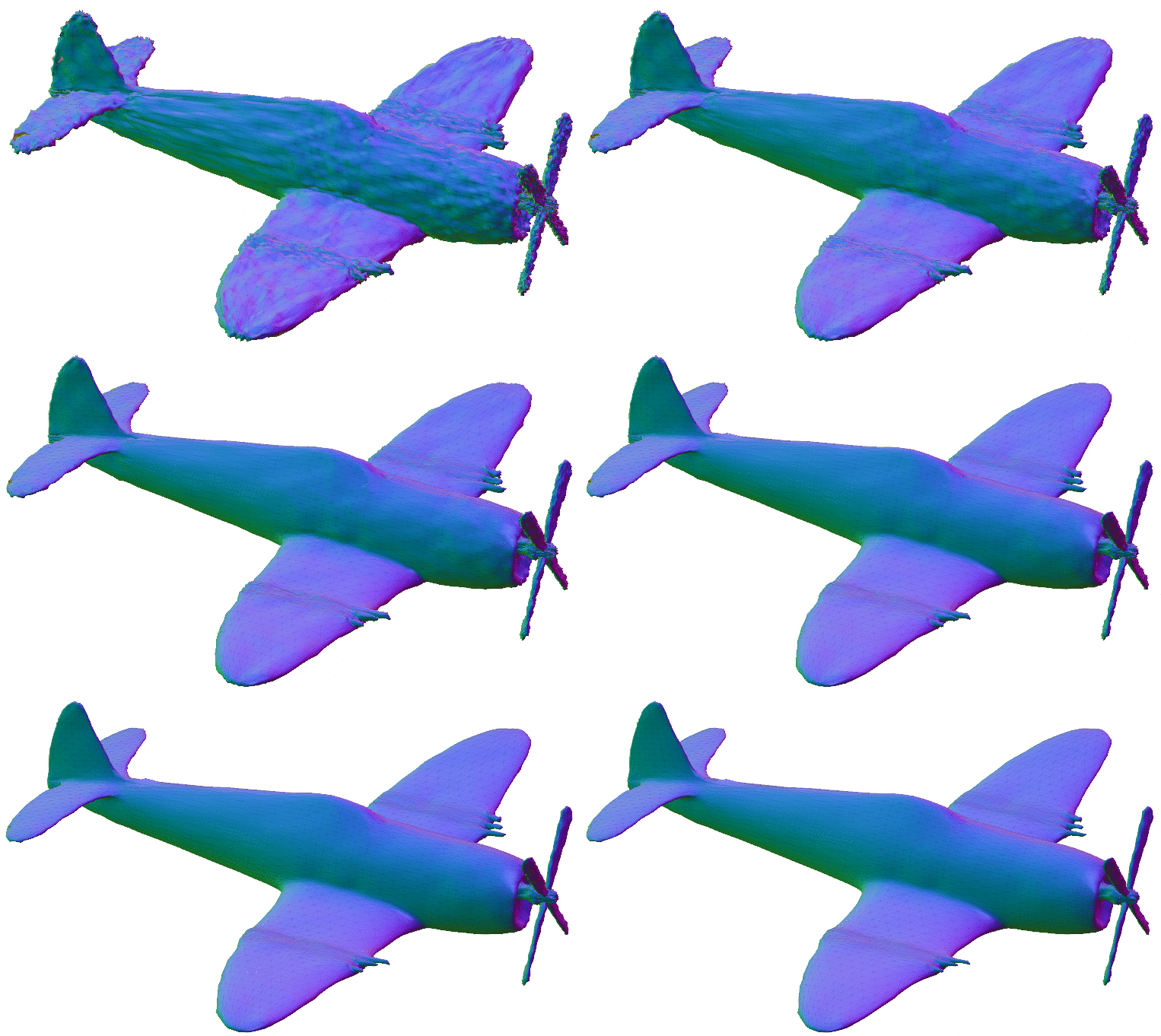
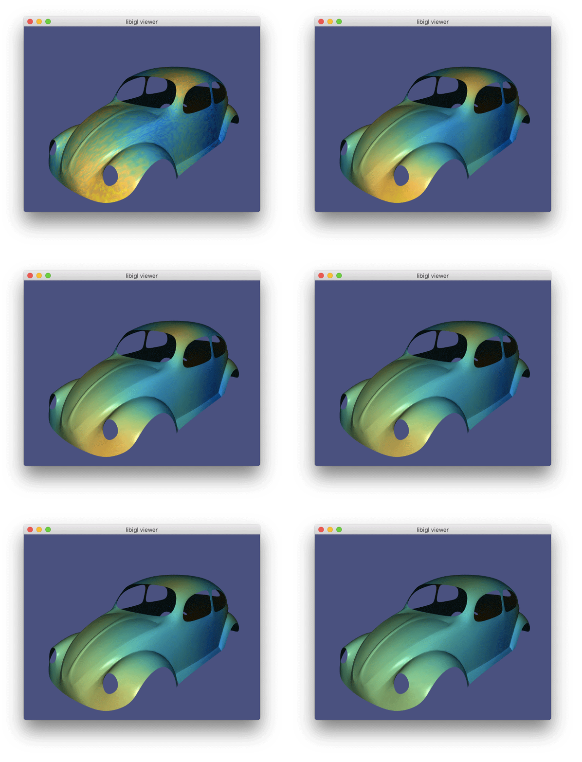
In this assignment we will explore how to smooth a data signal defined over a curved surface. The data signal may be a scalar field defined on a static surface: for example, noisy temperatures on the surface of an airplane. Smoothing in this context can be understood as data denoising:

The signal could also be the geometric positions of the surface itself. In this context, smoothing acts also affects the underlying geometry of the domain. We can understand this operation as surface fairing:

Flow-based formulation

In both cases, the underlying mathematics of both operations will be very similar. If we think of the signal as undergoing a flow toward a smooth solution over some phony notion of "time", then the governing partial differential equation we will start with sets the change in signal value $u$ over time proportional to the Laplacian of the signal $∆u$ (for now, roughly the second derivative of the signal as we move on the surface):

\[ \frac{∂ u}{∂ t} = λ ∆ u, \]

where the scalar parameter $λ$ controls the rate of smoothing.

When the signal is the surface geometry, we call this a geometric flow.

There are various ways to motivate this choice of flow for data-/geometry-smoothing. Let us consider one way that will introduce the Laplacian as a form of local averaging.

Given a noisy signal $f$, intuitively we can smooth $f$ by averaging every value with its neighbors' values. In continuous math, we might write that the smoothed value $u(\x)$ at any point on our surface $\x ∈ \S$ should be equal to the average value of some small ball of nearby points:

\[ u(\x) = \frac{1}{|B(\x))|} ∫_{B(\x)} f(\z) ;d\z, \]

If the ball $B(\x)$ is small, then we will have to repeat this averaging many times to see a global smoothing effect. Hence, we can write that the current value $u^t$ flows toward smooth solution by small steps $δt$ in time:

\[ u^{t+δt}(\x) = \frac{1}{|B(\x))|} ∫_{B(\x)} u^t(\z) ;d\z. \]

Subtracting the current value $u^t(\x)$ from both sides and introducing a flow-speed parameter $λ$ we have a flow equation describing the change in value as an integral of relative values:

\[ \frac{∂ u}{∂ t} = λ \frac{1}{|B(\x))|} ∫_{B(\x)} (u(\z)-u(\x)) ;d\z. \]

For harmonic functions, $∆u =0$, this integral becomes zero in the limit as the radius of the ball shrinks to zero via satisfaction of the mean value theorem. It follows for a non-harmonic $∆u ≠ 0$ this integral is equal to the Laplacian of the $u$, so we have arrived at our flow equation:

\[ \frac{∂ u}{∂ t} = \lim_{|B(\x)| → 0} λ \frac{1}{|B(\x))|} ∫_{B(\x)} (u(\z)-u(\x)) ;d\z = λ ∆ u. \]

Energy-based formulation

Alternatively, we can think of a single smoothing operation as the solution to an energy minimization problem. If $f$ is our noisy signal over the surface, then we want to find a signal $u$ such that it simultaneously minimizes its difference with $f$ and minimizes its variation over the surface:

\[ u^* = \argmin_u E_(u)

\argmin_u ½∫_\S ( \underbrace{(f-u)²}\text{data} + \underbrace{λ‖∇u‖²}\text{smoothness} );dA, \]

where again the scalar parameter $λ$ controls the rate of smoothing. This energy-based formulation is equivalent to the flow-based formulation. Minimizing these energies is identical to stepping forward one temporal unit in the flow.

Calculus of variations

In the smooth setting, our energy $E$ is a function that measures scalar value of a given function u, making it a functional. To understand how to minimize a functional with respect to an unknown function, we will need concepts from the calculus of variations.

We are used to working with minimizing quadratic functions with respect to a discrete set of variables, where the minimum is obtained when the gradient of the energy with respect to the variables is zero.

In our case, the functional $E(u)$ is quadratic in $u$ (recall that the gradient operator $∇$ is a linear operator). The function $u$ that minimizes $E(u)$ will be obtained when any small change or variation in $u$ has no change on the energy values. To create a small change in a function $u$ we will add another function $v$ times a infinitesimal scalar $ε$. If $E(u)$ is minimized for a function $w$ and we are given another arbitrary function $v$, then let us define a function new function

\[ Φ(ε) = E(w+εv) = ½∫_\S ((f-w+εv)² + λ ‖∇w + ε∇v‖²) ;dA, \] where we observe that $Φ$ is quadratic in $ε$.

Since $E(w)$ is minimal then $Φ$ is minimized when $ε$ is zero, and if $Φ$ is minimal at $ε=0$, then the derivative of $Φ$ with respect $ε$ must be zero:

\[ \begin{align} 0 & = \left.\frac{∂Φ}{∂ε} \right|{ε = 0},\ & = \left.\frac{∂}{∂ε} ½∫\S ( (f-w-εv)² + λ ‖∇w + ε∇v‖²);dA, \right|{ε = 0} \ & = \left.\frac{∂}{∂ε} ½∫\S ( f^2 - 2wf - 2εfv +w²+2εvw +ε²v² + λ ‖∇w‖² + λ2ε∇v⋅∇w + λ ε²‖∇w‖²) ;dA \right|{ε = 0}\ & = \left.∫\S (-fv + vw +2εvw + λ∇v⋅∇w + λ ε‖∇w‖²) ;dA \right|{ε = 0}\ & = ∫\S (v(w-f) + λ∇v⋅∇w );dA. \end{align} \]

The choice of "test" function $v$ was arbitrary, so this must hold for any (reasonable) choice of $v$:

\[ 0 = ∫_\S (v(w-f) + λ∇v⋅∇w) ;dA \quad ∀ v. \]

It is difficult to claim much about $w$ from this equation directly because derivatives of $v$ are still involved. We can move a derivative from $v$ to a $w$ by applying Green's first identity:

\[ 0 = ∫_\S (v(w-f) - λv∆w );dA \quad (+ \text{boundary term} )\quad ∀ v, \] where we choose to ignore the boundary terms (for now) or equivalently we agree to work on closed surfaces $\S$.

Since this equality must hold of any $v$ let us consider functions that are little "blips" centered at any arbitrary point $\x ∈ \S$. A function $v$ that is one at $\x$ and quickly decays to zero everywhere else. To satisfy the equation above at $\x$ with this blip $v$ we must have that:

\[ w(\x)-f(\x) = λ∆w(\x). \] The choice of $\x$ was arbitrary so this must hold everywhere.

Because we invoke variations to arrive at this equation, we call the energy-based formulation a variational formulation.

Implicit smoothing iteration

Now we understand that the flow-based formulation and the variational formulation lead to the same system, let us concretely write out the implicit smoothing step.

Letting $u^0 = f$ we compute a new smoothed function $u^{t+1}$ given the current solution $u^t$ by solving the linear system of equations:

\[ u^t(\x) = (\text{id}-λ∆)u^{t+1}(\x), \quad ∀ \x ∈ \S \] where $\text{id}$ is the identity operator. In the discrete case, we will need discrete approximations of the $\text{id}$ and $∆$ operators.

Discrete Laplacian

There are many ways to derive a discrete approximation of the Laplacian $∆$ operator on a triangle mesh using:

• finite volume method,
  • "The solution of partial differential equations by means of electrical networks" [MacNeal 1949, pp. 68],
  • "Discrete differential-geometry operators for triangulated 2-manifolds" [Meyer et al. 2002],
  • Polygon mesh processing [Botsch et al. 2010],
• finite element method,
  • "Variational methods for the solution of problems of equilibrium and vibrations" [Courant 1943],
  • Algorithms and Interfaces for Real-Time Deformation of 2D and 3D Shapes [Jacobson 2013, pp. 9]
• discrete exterior calculus
  • Discrete Exterior Calculus [Hirani 2003, pp. 69]
  • Discrete Differential Geometry: An Applied Introduction [Crane 2013, pp. 71]
• gradient of surface area → mean curvature flow
  • "Computing Discrete Minimal Surfaces and Their Conjugates" [Pinkall & Polthier 1993]

All of these techniques will produce the same sparse Laplacian matrix $\L ∈ \R^{n×n}$ for a mesh with $n$ vertices.

Finite element derivation of the discrete Laplacian

We want to approximate the Laplacian of a function $∆u$. Let us consider $u$ to be piecewise-linear represented by scalar values at each vertex, collected in $\u ∈ \R^n$.

Any piecewise-linear function can be expressed as a sum of values at mesh vertices times corresponding piecewise-linear basis functions (a.k.a hat functions, $φ_i$):

\[ \begin{align} u(\x) &= ∑_{i=1}^n u_i φ_i(\x), \ φ(\x) &= \begin{cases} 1 & \text{if $\x = \v_i$}, \ \frac{\text{Area($\x$,$\v_j$,$\v_k$)}}{\text{Area($\v_i$,$\v_j$,$\v_k$)}} & \text{if $\x ∈ \text{triangle}(i,j,k)$}, \ 0 & \text{otherwise}. \end{cases} \end{align} \]

By plugging this definition into our smoothness energy above, we have discrete energy that is quadratic in the values at each mesh vertex:

\[ \begin{align} ∫_\S ‖∇u(\x)‖² ;dA
&= ∫_\S \left|∇\left(∑_{i=1}^n u_i φ_i(\x)\right)\right|^2 ;dA \ &= ∫_\S \left(∑_{i=1}^n u_i ∇φ_i(\x)\right)⋅\left(∑_{i=1}^n u_i ∇φ_i(\x)\right) ;dA \ &= ∫_\S ∑_{i=1}^n ∑_{j=1}^n ∇φ_i⋅∇φ_j u_i u_j ;dA \ &= \u^\transpose \L \u, \quad \text{where } L_{ij} = ∫_\S ∇φ_i⋅∇φ_j ;dA. \end{align} \]

By defining $φ_i$ as piecewise-linear hat functions, the values in the system matrix $L_{ij}$ are uniquely determined by the geometry of the underlying mesh. These values are famously known as cotangent weights. "Cotangent" because, as we will shortly see, of their trigonometric formulae and "weights" because as a matrix $\L$ they define a weighted graph Laplacian for the given mesh. Graph Laplacians are employed often in geometry processing, and often in discrete contexts ostensibly disconnected from FEM. The choice or manipulation of Laplacian weights and subsequent use as a discrete Laplace operator has been a point of controversy in geometry processing research (see "Discrete laplace operators: no free lunch" [Wardetzky et al. 2007]).

We first notice that $∇φ_i$ are constant on each triangle, and only nonzero on triangles incident on node $i$. For such a triangle, $T_α$, this $∇φ_i$ points perpendicularly from the opposite edge $e_i$ with inverse magnitude equal to the height $h$ of the triangle treating that opposite edge as base: \begin{equation} |∇φ_i| = \frac{1}{h} = \frac{|\e_i|}{2A}, \end{equation} where $\e_i$ is the edge $e_i$ as a vector and $A$ is the area of the triangle.

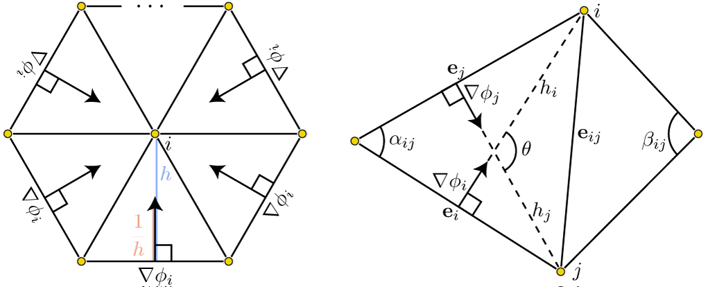
Now, consider two neighboring nodes $i$ and $j$, connected by some edge $\e_{ij}$. Then $∇φ_i$ points toward node $i$ perpendicular to $\e_i$ and likewise $∇ φ_j$ points toward node $j$ perpendicular to $\e_j$. Call the angle formed between these two vectors $θ$. So we may write:

\[ ∇ φ_i ⋅ ∇ φ_j = |∇ φ_i| |∇ φ_j| \cos θ = \frac{|\e_j|}{2A}\frac{|\e_i|}{2A} \cos θ. \]

Now notice that the angle between $\e_i$ and $\e_j$, call it $α_{ij}$, is $π - θ$, but more importantly that: \[ \cos θ = - \cos \left(π - θ\right) = -\cos α_{ij}. \] So, we can rewrite equation the cosine law equation above into: \[ -\frac{|\e_j|}{2A}\frac{|\e_i|}{2A} \cos α_{ij}. \] Now, apply the definition of sine for right triangles: \[ \sin α_{ij} = \frac{h_j}{|\e_i|} = \frac{h_i}{|\e_j|}, \] where $h_i$ is the height of the triangle treating $\e_i$ as base, and likewise for $h_j$. Rewriting the equation above, replacing one of the edge norms, e.g.\ $|\e_i|$: \[ -\frac{|\e_j|}{2A} \frac{\frac{h_j}{\sinα_{ij}}}{2A} \cos α_{ij}. \]

Combine the cosine and sine terms: \[ -\frac{|\e_j|}{2A} \frac{h_j}{2A} \cot α_{ij}. \]

Finally, since $|\e_j|h_j=2A$, our constant dot product of these gradients in our triangle is: \[ ∇ φ_i ⋅ ∇ φ_j = -\frac{\cot α_{ij}}{2A}. \]

Similarly, inside the other triangle $T_β$ incident on nodes $i$ and $j$ with angle $β_{ij}$ we have a constant dot product: \[ ∇ φ_i ⋅ ∇ φ_j = -\frac{\cot β_{ij}}{2B}, \] where $B$ is the area $T_β$.

Recall that $φ_i$ and $φ_j$ are only both nonzero inside these two triangles, $T_α$ and $T_β$. So, since these constants are inside an integral over area we may write: \[ \int\limits_\S ∇ φ_i ⋅ ∇ φ_j ;dA = \left.A∇ φ_i ⋅ ∇ φ_j \right|{T_α} + \left.B∇ φ_i ⋅ ∇ φ_j \right|{T_β}

-\frac{1}{2} \left( \cot α_{ij} + \cot β_{ij} \right). \]

Mass matrix

Treated as an operator (i.e., when used multiplied against a vector $\L\u$), the Laplacian matrix $\L$ computes the local integral of the Laplacian of a function $u$. In the energy-based formulation of the smoothing problem this is not an issue. If we used a similar FEM derivation for the data term we would get another sparse matrix $\M ∈ \R^{n × n}$:

\[ ∫_\S (u-f)² ;dA = ∫_\S ∑_{i=1}^n ∑_{j=1}^n φ_i⋅φ_j (u_i-f_i) (u_j-f_j) ;dA = (\u-\f)^\transpose \M (\u-\f), \] where $\M$ as an operator computes the local integral of a function's value (i.e., $\M\u$).

This matrix $\M$ is often diagonalized or lumped into a diagonal matrix, even in the context of FEM. So often we will simply set:

\[ M_{ij} = \begin{cases} ⅓ ∑_{t=1}^m \begin{cases} \text{Area}(t) & \text{if triangle $t$ contains vertex $i$} \ 0 & \text{otherwise} \end{cases} & \text{if $i=j$}\ 0 & \text{otherwise}, \end{cases} \] for a mesh with $m$ triangles.

If we start directly with the continuous smoothing iteration equation, then we have a point-wise equality. To fit in our integrated Laplacian $\L$ we should convert it to a point-wise quantity. From a units perspective, we need to divide by the local area. This would result in a discrete smoothing iteration equation:

\[ \u^t = (\I - λ\M^{-1} \L)\u^{t+1}, \]

where $\I ∈ \R^{n×n}$ is the identity matrix. This equation is correct but the resulting matrix $\A := \I - λ\M^{-1} \L$ is not symmetric and thus slower to solve against.

Instead, we could take the healthier view of requiring our smoothing iteration equation to hold in a locally integrated sense. In this case, we replace mass matrices on either side:

\[ \M \u^t = (\M - λ\L)\u^{t+1}. \]

Now the system matrix $\A := \M + λ\L$ will be symmetric and we can use Cholesky factorization to solve with it.

Laplace Operator is Intrinsic

The discrete Laplacian operator and its accompanying mass matrix are intrinsic operators in the sense that they only depend on lengths. In practical terms, this means we do not need to know where vertices are actually positioned in space (i.e., $\V$). Rather we only need to know the relative distances between neighboring vertices (i.e., edge lengths). We do not even need to know which dimension this mesh is living in.

This also means that applying a transformation to a shape that does not change any lengths on the surface (e.g., bending a sheet of paper) will have no affect on the Laplacian.

Data denoising

For the data denoising application, our geometry of the domain is not changing only the scalar function living upon it. We can build our discrete Laplacian $\L$ and mass matrix $\M$ and apply the above formula with a chosen $λ$ parameter.

Geometric smoothing

For geometric smoothing, the Laplacian operator (both $∆$ in the continuous setting and $\L,\M$ in the discrete setting) depend on the geometry of the surface $\S$. So if the signal $u$ is replaced with the positions of points on the surface (say, $\V ∈ \R^{n×3}$ in the discrete case), then the smoothing iteration update rule is a non-linear function if we write it as:

\[ \M^{t+1} \V^t = (\M^{t+1} - λ\L^{t+1})\V^{t+1}. \]

However, if we assume that small changes in $\V$ have a negligible effect on $\L$ and $\M$ then we can discretize explicitly by computing $\L$ and $\M$ before performing the update:

\[ \M^{t} \V^t = (\M^{t} - λ\L^{t}) \V^{t+1}. \]

Why did my mesh disappear?

Repeated application of geometric smoothing may cause the mesh to "disappear". Actually the updated vertex values are being set to NaNs due to degenerate numerics. We are rebuilding the discrete Laplacian at every new iteration, regardless of the "quality" of the mesh's triangles. In particular, if a triangle tends to become skinnier and skinnier during smoothing, what will happen to the cotangents of its angles?

In "Can Mean-Curvature Flow Be Made Non-Singular?", Kazhdan et al. derive a new type of geometric flow that is stable (so long as the mesh at time $t=0$ is reasonable). Their change is remarkably simple: do not update $\L$, only update $\M$.

Tasks

Learn an alternative derivation of cotangent Laplacian

The "cotangent Laplacian" by far the most important tool in geometry processing. It comes up everywhere. It is important to understand where it comes from and be able to derive it (in one way or another).

The background section above contains a FEM derivation of the discrete "cotangnet Laplacian". For this (unmarked) task, read and understand one of the other derivations listed above.

Hint: The finite-volume method used in [Botsch et al. 2010] is perhaps the most accessible alternative.

White list

• igl::doublearea
• igl::edge_lengths

Black list

• igl::cotmatrix_entries
• igl::cotmatrix
• igl::massmatrix
• Trig functions sin, cos, tan etc. (e.g., from #include <cmath>) See background notes about "intrinisic"-ness

src/cotmatrix.cpp

Construct the "cotangent Laplacian" for a mesh with edge lengths l. Each entry in the output sparse, symmetric matrix L is given by:

\[ L_{ij} = \begin{cases} ½ \cot{α_{ij}} + ½ \cot{β_{ij}} & \text{if edge $ij$ exists} \ - ∑_{j≠i} L_{ij} & \text{if $i = j$} \ 0 & \text{otherwise} \end{cases} \]

Hint: Review the law of sines and law of cosines and Heron's ancient formula to derive a formula for the cotangent of each triangle angle that only uses edge lengths.

src/massmatrix.cpp

Construct the diagonal(ized) mass matrix M for a mesh with given face indices in F and edge lengths l.

src/smooth.cpp

Given a mesh (V,F) and data specified per-vertex (G), smooth this data using a single implicit Laplacian smoothing step.

This data could be a scalar field on the surface and smoothing corresponds to data denoising.

Or the data could be the vector field of the surface's own geometry. This corresponds to geometric smoothing.