In this project, we use convolutional neural networks to classify traffic signs. We train and validate a model so it can classify traffic sign images using the German Traffic Sign Dataset.
What was the first architecture that was tried and why was it chosen?
The first architecture tried was LeNet-5. It was chosen because it was the architecture explained through the course material.
What were some problems with the initial architecture?
The initial architecture for LeNet-5 had a channel depth of 1 and output of 10. Moreover, there were no dropout layers to avoid overfitting.
How was the architecture adjusted and why was it adjusted?
The input channel depth was increased to 3, output was set to 43 because we have 43 different labels to identify. Adding a dropout layer was tried.
Which parameters were tuned? How were they adjusted and why?
The learning rate was increased to 0.002 for faster convergence.
What are some of the important design choices and why were they chosen?
Instead of modifying the architecture, I choose to combine and reshuffle the data. Better approach would have been to create more data using image augmentation techniques and then add dropout layers to avoid overfitting.
I used the NumPy library to calculate summary statistics of the traffic signs data set:
- The size of training set is 34799
- The size of the validation set is 4410
- The size of test set is 12630
- The shape of a traffic sign image is 32x32x3
- The number of unique classes/labels in the data set is 43
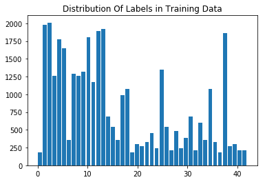
Here is an exploratory visualization of the data set. It is a histogram showing how the data is distributed between 43 labels
As part of the preprocessing step, I combined all the dataset and reshuffled to generate the training, validation and testing datasets using the train_test_split function. Follwed by normalizing the data so the data has close to zero mean and equal variance. In future, I would like to experiment with data augmentation to generate additional data. As seen in the above histogram, the distribution of data between various labels is uneven. We could use data augmentation to balance it out and that would help produce even better results.
I started with the default LeNet-5 architecture and played around with adding Dropout layers which didn't seem to help much with the accuracy. My final model consisted of the following layers:
| Layer | Description |
|---|---|
| Input | 32x32x3 RGB image |
| Convolution 5x5 | 1x1 stride, valid padding, outputs 28x28x6 |
| RELU | |
| Max pooling | 2x2 stride, valid padding, outputs 14x14x6 |
| Convolution 5x5 | 1x1 stride, valid padding, outputs 10x10x16 |
| RELU | |
| Max pooling | 2x2 stride, valid padding, outputs 5x5x16 |
| Flatten | outputs 400 |
| Fully Connected | outputs 120 |
| RELU | |
| Fully Connected | outputs 84 |
| RELU | |
| Fully Connected | outputs 43 |
| Softmax |
To train the model, I used an adam optimizer, with a batch size of 256, learning rate of 0.002, running it for 10 epochs.
I followed an iterative approach converging to an accuracy > 0.93. Since I already had an implementation for the LeNet-5 architecture, I just went ahead with that in the beginning by just modifying the image channel depth to 3. Later, more fully connected layers were added to the bottom and a dropout layer with a 0.9 dropout was also included in between these fully connected layers. But this did not help increase the accuracy, so I reverted back to the original architecture. What helped was shuffling and normalizing of data in the pre-processing stages. The learning rate hyperparameter was increased from 0.001 to 0.002 for faster convergence since I observed that with the default learning rate, it required more number of epochs to reach the optimum accuracy.
My final model results were:
- validation set accuracy of 97.4%
- test set accuracy of 97.5%
Since, the validation set accuracy is very close to the test set accuracy, the model is working well. In future, data augmentation coupled with a droupout layer should help increase the accuracy.
Below are five German traffic signs that I found on the web:
The last image might be difficult to classify because of its low contrast ratio.
Here are the results of the prediction:
| Image | Prediction |
|---|---|
| Dangerous curve to the right | Dangerous curve to the right |
| Keep right | Keep right |
| No passing | No passing |
| Priority road | Priority road |
| Roundabout mandatory | Roundabout mandatory |
The model was able to correctly guess 5 of the 5 traffic signs, which gives an accuracy of 100%. This compares favorably to the accuracy on the test set of 97.2%
The code for making predictions on my final model is located in the 9th cell of the Ipython notebook. For the first image, the model is sure that this is a Dangerous curve to the right sign (probability of 1.0), and the image does contain a stop sign. The last image was relatively difficult to classify due to the low contrast. But the model could predict it with a probability of 0.94. The top five soft max probabilities were:
| Probability | Prediction |
|---|---|
| 1.00 | Dangerous curve to the right |
| 1.00 | Keep right |
| 1.00 | No passing |
| 1.00 | Priority road |
| 0.95 | Roundabout mandatory |


