Detecting targets using simulated radar measurements

Steps

Designing wave

d_res = 1;
speed_of_light = 3*10^8;  % 3e8
RMax = 200;

Bsweep = speed_of_light / (2 * d_res);  % bandwidth
Tchirp = 5.5 * 2 * RMax / speed_of_light; % chirp time
alpha = Bsweep / Tchirp; % slope of FMCW chirps
fc = 77e9;              % carrier frequency of radar 
                                                    
Nd = 128;                % number of chirps in one sequence
Nr = 1024;               % number of samples on each chirp    

t = linspace(0, Nd * Tchirp, Nr * Nd); % total time for samples

% vectors for Tx, Rx and Mix based on the total samples input
Tx = zeros(1, length(t));    % transmitted signal
Rx = zeros(1, length(t));    % received signal
Mix = zeros(1, length(t));   % beat signal

% vectors for range covered and time delay
r_t = zeros(1, length(t));
td = zeros(1, length(t));

%% Signal generation and Moving Target simulation
% Running the radar scenario over the time. 

for i = 1:length(t)         
    % for each timestamp update the range of the target for constant velocity
    r_t(i) = d0 + v0 * t(i);
    td(i) = 2 * r_t(i) / speed_of_light;
    
    % for each time sample update the transmitted and received signal
    Tx(i) = cos(2 * pi * (fc * t(i) + alpha * t(i)^2 / 2));
    Rx(i) = cos(2 * pi * (fc * (t(i) - td(i)) + (alpha * (t(i) - td(i))^2) / 2));
    
    % now by mixing the transmit and receive generate the beat signal by performing
    % element-wise matrix multiplication of transmit and receiver signal
    Mix(i) = Tx(i) .* Rx(i);  % beat signal
end

FFT

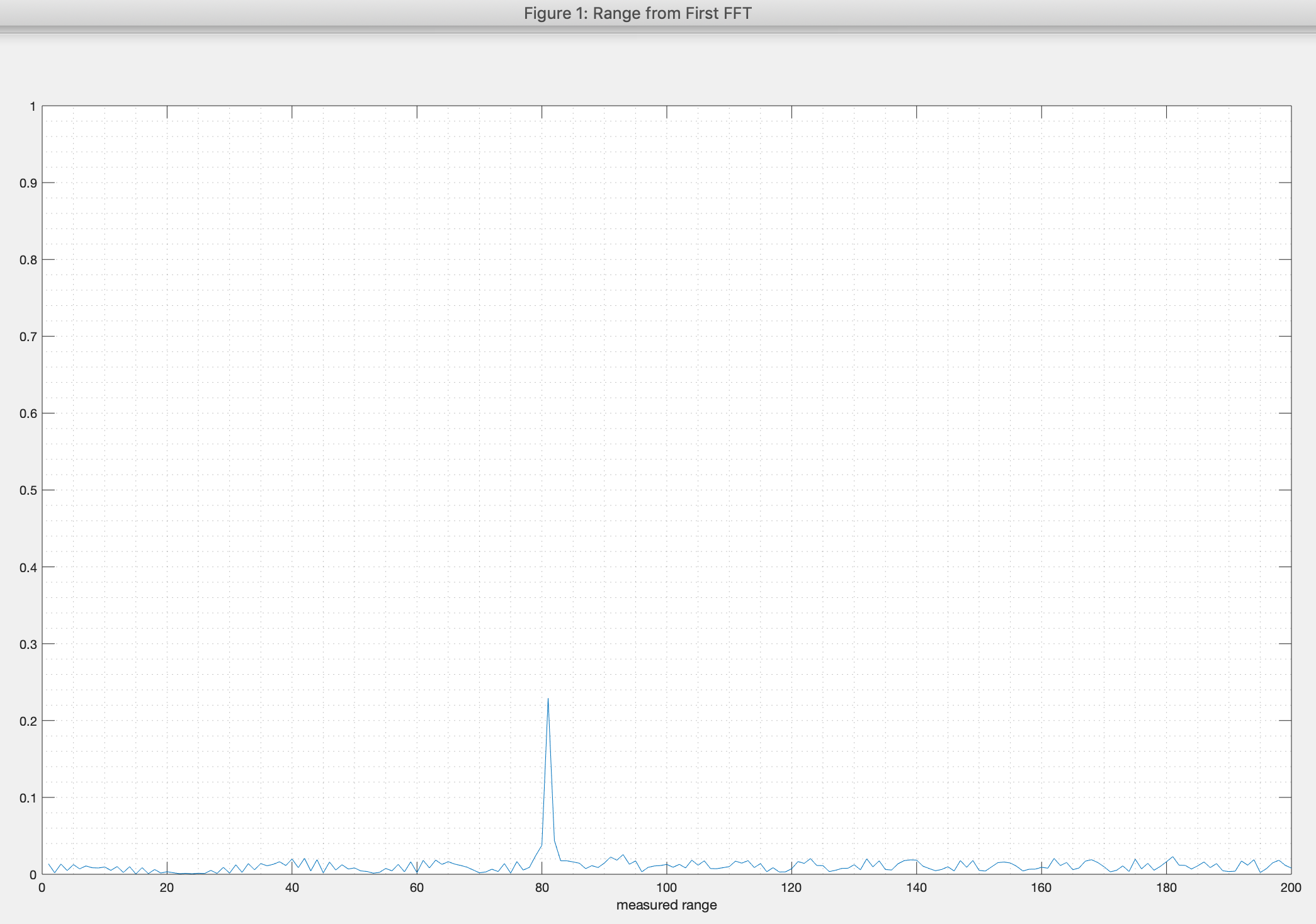
%% RANGE (1st FFT)

% running the Fast Fourier Transform (FFT) on the beat signal along the range bins dimension (Nr) and normalise
sig_fft = fft(Mix, Nr) ./ Nr;

% taking absolute value of FFT output
sig_fft = abs(sig_fft);       

% output of FFT is double-sided signal, but since we are interested in one side of the spectrum only, we throw out half of the samples
sig_fft = sig_fft(1 : (Nr / 2));

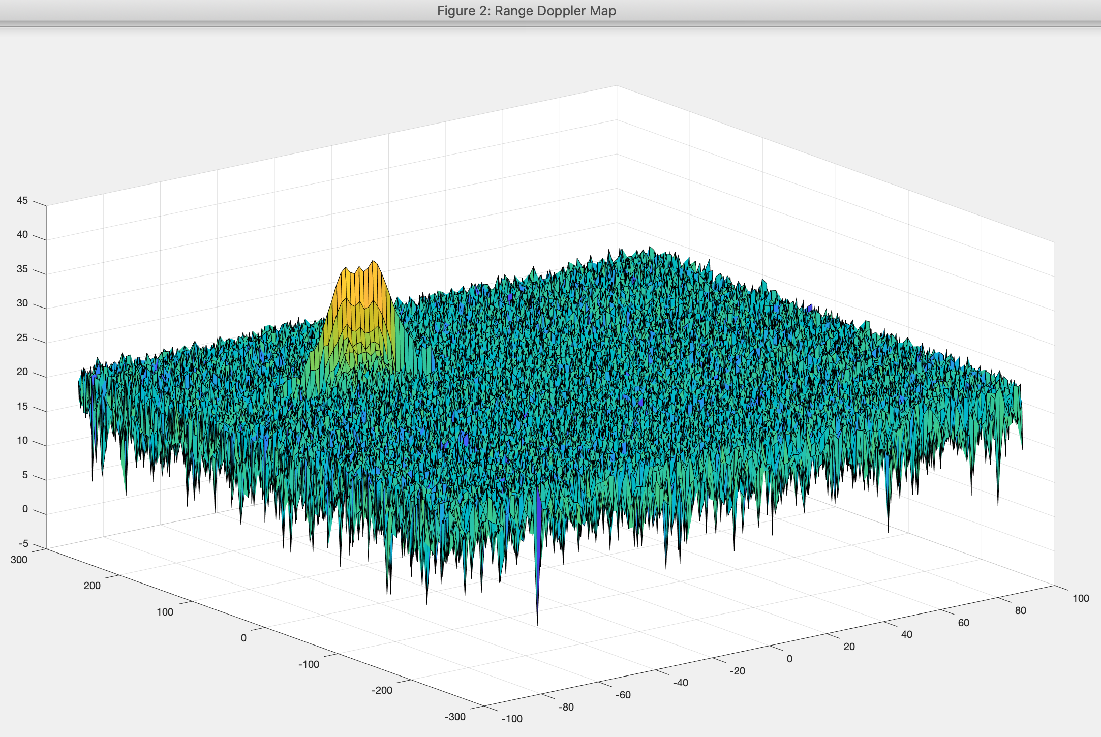
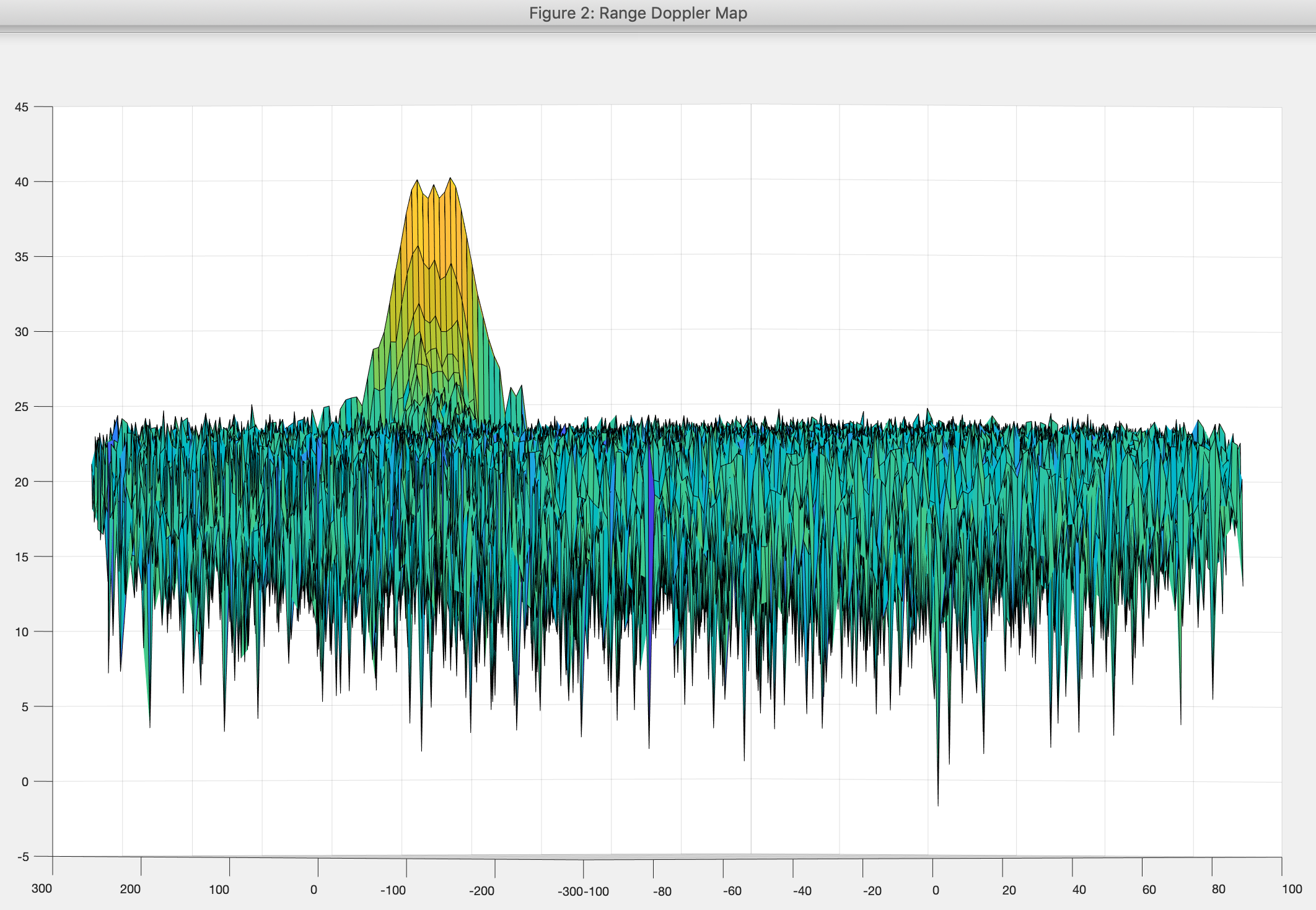
%% VELOCITY (2nd FFT)

Mix = reshape(Mix, [Nr, Nd]);

% 2D FFT using the FFT size for both dimensions
sig_fft2 = fft2(Mix, Nr, Nd);

% taking just one side of signal from range dimension
sig_fft2 = sig_fft2(1 : Nr / 2, 1 : Nd);
sig_fft2 = fftshift(sig_fft2);
RDM = abs(sig_fft2);
RDM = 10*log10(RDM);

Selecting training, guard cells and offset

% selecting number of training cells in both the dimensions by trial and error trying to match objective
Tcr = 10;
Tcd = 4;

% selecting number of guard cells in both dimensions around the Cell Under Test (CUT) for accurate estimation
Gcr = 5;
Gcd = 2;

% offsetting the threshold by signal-to-noise-ratio (SNR) value in dB
offset = 1.4;

% creating vector to store noise level for each iteration on training cells
noise_level = zeros(Nr / 2 - 2 * (Tcd + Gcd), Nd - 2 * (Tcr + Gcr));
gridSize = (2 * Tcr + 2 * Gcr + 1) * (2 * Tcd + 2 * Gcd + 1);
trainingCellsNum = gridSize - (2 * Gcr + 1) * (2 * Gcd + 1);

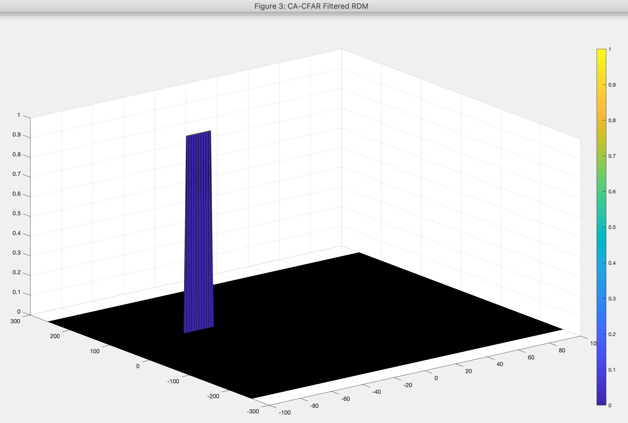
Suppressing the non-thresholded cells at the edges

Generating a thresholded block, which is smaller than the Range Doppler Map as the CUT cannot be located at the edges of matrix. Hence, few cells will not be thresholded. To keep the map size same set those values to 0

CFAR_sig = zeros(size(RDM));

% Using RDM[x,y] as the matrix from the output of 2D FFT for implementing CFAR
for j = 1 : Nd - 2 * (Tcr + Gcr)
    for i = 1 : Nr / 2 - 2 * (Tcd + Gcd)

maggieliuzzi/radar_target_simulation_and_detection

Detecting targets using simulated radar measurements

Steps