Estimating epistatic interactions from SARS-CoV-2 genomes, using mutual information
This repository contains the code used to estimate epistatic interactions from multiple sequence alignments (MSAs) of SARS-CoV-2 genomes, using a mutual information (MI) based method.
The code assumes that the data comes from the GISAID repository, although it will solely focus on sequences that are also in public repositories.
Clone this repository, including submodules
git clone --recursive git@github.com:microbial-pangenomes-lab/2022_sarscov2_epistasis.git
For convenience all necessary software packages can be installed using the provided conda environment file:
mamba env create -f environment.yml
conda activate epistasis
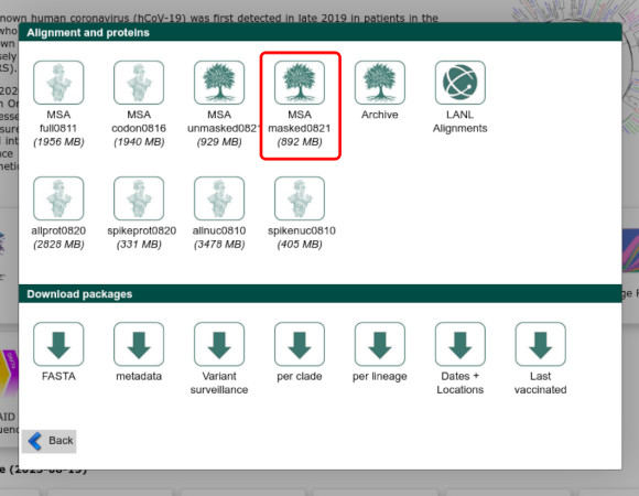
If you have an account on GISAID, head over to the SARS-CoV-2 page and go to the "Downloads" screen. Get the MSA by clicking on the "MSA masked" button.
In the example above this means you will obtain an archive called mmsa_2023-08-21.tar.xz, which you should
place in the repository root directory.
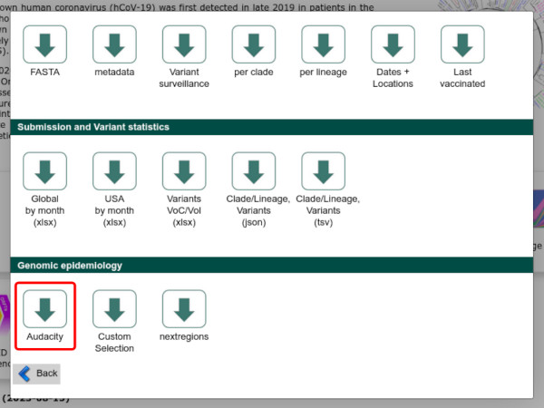
From the same "Downloads" screen, scroll down to the "Genomic epidemiology" section and click on the "Audacity"
button. In the next screen click on the "Download tree" button. In the example above you will obtain a file called GISAID-hCoV-19-phylogeny-2023-08-17.zip,
which should also be placed in the repository root directory.
The first step is to subset the MSA to those samples that are present in both the phylogenetic tree
and public repositories. Unfortunately this means that the MSA has to be fully inflated, as there does not seem to be a way to stream a single file from a .xz archive.
bash 01_preprocess.sh GISAID-hCoV-19-phylogeny-2023-08-17.zip mmsa_2023-08-21.tar.xz 16
In the above example we have selected 16 cores to handle inflation/deflation of the MSAs.
As output we have obtained a filtered MSA called prefiltered.fasta.xz.
The second step is to split the dataset in two ways: smaller subsets of 1,000, 10,000, 100,000 and 1,000,000 random sequences, and time resolved subsets, one for each month until a defined cutoff.
bash 02_split.sh 16 GISAID-hCoV-19-phylogeny-2023-08-17/metadata.csv 2023-03
In the above example we are using 16 cores to deflate the generated MSAs and to run nextclade on
each time-resolved subset. One subset with 2,500 sequences per month will be generated
from February 2020 until March 2023 (2023-03). The following directories will be created:
data/subsetswith the smaller subsets (i.e.1000.fasta.xz,10000.fasta.xz, ...)data/time/with one MSA per month (i.e.2020-02.fasta.xz,2020-03.fasta.xz, ...)data/time-filtered/with one MSA per month, after removal of known "bad sequences"out/time-lineages/with one nextclade output per month (i.e.2020-02.tsv,2020-03.tsv, ...)
The third step must be repeated multiple times, one for each time resolved subset. It will concatenate all subsets prior to the focal one in a single file; for instance:
bash 03_prepare_time_subset.sh 2020-05
Will concatenate the MSA for 2020-02, 2020-03, 2020-04, and 2020-05 into a single one, and
place it in the data/time-filtered-subsets directory under the name 2020-05.fasta.xz.
The fourth step is the actual computation of MI values, and must be repeated for each subset. For example for the complete dataset the command is:
bash 04_run.sh GISAID-hCoV-19-phylogeny-2023-08-17.zip 16 prefiltered.fasta.xz out/all-notime
Which will use 16 cores (and more than 200Gb of RAM) and place all outputs in the
out/all-notime directory. To speed up this step for the complete dataset we submitted one src/spydrpick_alt.py job to a HPC separately. The two important output files are mi_annotated.tsv.gz (annotated MI values) and mi_annotated_prefilter.tsv.gz (annotated MI values before filtering using the ARACNE algorithm).
For the time resolved subsets an extra argument indicating the final month to consider must be added, so that the time-weighting can be applied.
bash 04_run.sh GISAID-hCoV-19-phylogeny-2023-08-17.zip 16 data/time-filtered-subsets/2022-12.fasta.xz out/time-filtered-subsets/2022-12/ 2022-12
The next step is to run Direct Coupling Analysis using the plmc implementation. Compile it first:
cd plmc
make all-openmp
cd ..
And then run it on the Spike portion of any MSA of choice:
bash 05_plmc.sh data/time-filtered-subsets/2023-03.fasta.xz out/spikes/2023-03 16
Which will use 16 cores and create the following files:
data/spikes/2023-03.fastawhich contains the nucleotide MSA for the Spike geneout/spikes/2023-03which contains two files (2023-03.ECand2023-03.params) as given byplmc.
All the plots shown in the manuscript have been generated through reproducible jupyter notebooks. Once all analyses have been run, download the necessary support file using the last bash script and then turn on a jupyter lab instance:
bash 07_reports.sh
jupyter lab
You can then run the notebooks one by one to regenerate all plots and supplementary material.
Innocenti, G., & Galardini, M. (2023). Real-time identification of epistatic interactions in SARS-CoV-2 from large genome collections (p. 2023.08.22.554253). bioRxiv. https://doi.org/10.1101/2023.08.22.554253
The method to compute mutual information has been first described in the following publication:
Pensar, J., Puranen, S., Arnold, B., MacAlasdair, N., Kuronen, J., Tonkin-Hill, G., ... & Corander, J. (2019). Genome-wide epistasis and co-selection study using mutual information. Nucleic acids research, 47(18), e112-e112.
and we made our own implementation following the one described in the panaroo repository:
Tonkin-Hill, G., MacAlasdair, N., Ruis, C., Weimann, A., Horesh, G., Lees, J. A., ... & Parkhill, J. (2020). Producing polished prokaryotic pangenomes with the Panaroo pipeline. Genome biology, 21, 1-21.

