Part 1: Data Wrangling
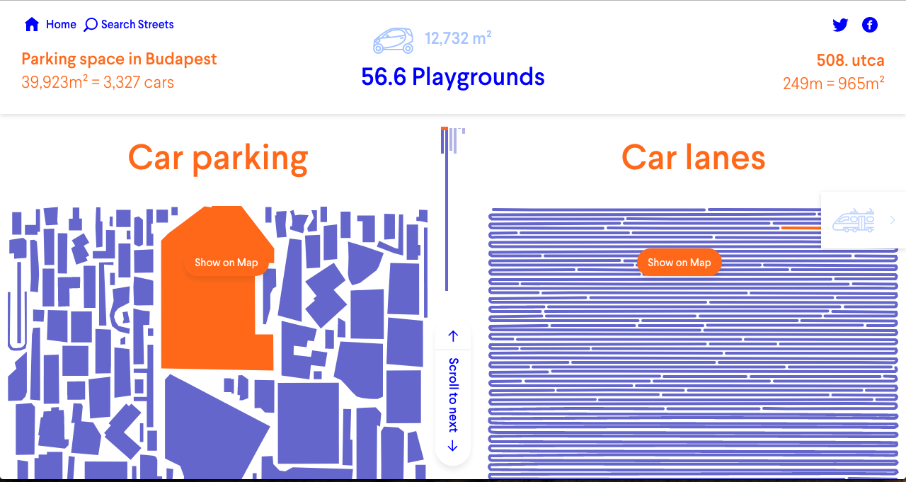
What the Street!? was derived out of the question “How do new and old mobility concepts change our cities?”. It was raised by Michael Szell and Stephan Bogner during their residency at moovel lab. With support of the lab team they set out to wrangle data of cities around the world to develop and design this unique mobility space report.
What the Street!? was made out of open-source software and resources. Thanks to the OpenStreetMap contributors and many other pieces we put together the puzzle of urban mobility space seen above.
Implemented project URL: https://whatthestreet.com/
Read more about the technical details behind What the Street!? on our blog https://move-lab.space/blog/about-what-the-street and in the scientific paper https://www.cogitatiopress.com/urbanplanning/article/view/1209/.
The complete codebase consist of two independent parts:
- Data Wrangling
- Front & Backend
This is part 1. It wrangles the OpenStreetMap data and creates the SVG files underlying the visuals of What the Street!?.
You can find part 2 here: https://github.com/mszell/whatthestreet
- Note about code quality
- Inital setup
- Adding a city
- Team
- Acknowledgements
The code in this repository was produced for the specific use case of wrangling data for What the Street!?. Since this is not live production code, but code to pre-process data, we did not strictly apply best practices of software development. The code grew organically together with various deadlines and requirements that came from front & backend develoment on the way. Nevertheless, we commented and documented as well as possible to make the process reproducible.
- Get NodeJS
- Get osmconvert.c. Set
border__edge_M 1300004so it can handle larger poly files. Compile:gcc osmconvert.c -lz -O3 -o osmconvert - Get osmfilter
- Get MongoDB
- Get QGIS, install the osmpoly_export plugin
- Get Anaconda (Python 3.*)
- Get SVGnest-batch
- Extra python libraries to install: pymongo, shapely, haversine, osmnx (first rtree!), pyprind
- Get mongosm from Stephan Bogner's fork, and in options.js of mongosm/lib, set
populateGeometry: false. To get dependencies, run:npm install
Follow this order. If not noted otherwise, run commands in terminal. Examples for Berlin.
- Get shapefile of city boundary from somewhere. If nowhere found, use Turbopass, mind the correct admin_level:
[out:json]; ( node[boundary="administrative"][admin_level=6](48.46, 8.79, 48.93, 9.50); way[boundary="administrative"][admin_level=6](48.46, 8.79, 48.93, 9.50); ) ;(._;>;); out skel;
- Load file into QGIS, save as a duplicate with correct
CRS: EPSG:4326, and save asberlin_boundary.polyviaVector > Export OSM Poly - Download and unpack osm.bz2 file that contains the city from geofabrik, e.g berlin-latest
- Crop osm file according the boundary using osmconvert
./osmconvert berlin-latest.osm -B=berlin_boundary.poly --drop-broken-refs -o=berlin_cropped.osm
- Load osm data into mongoDB via mongosm
node mongosm.js --max_old_space_size=8192 -db berlin_raw -f berlin_cropped.osm(don't forget to runnpm installbefore running the script the first time to install dependencies) - Set cityname parameter (in Jupyter notebook) and execute
01_generategeometries.ipynb
Note: osmfilter seems buggy and does not actually remove some things we want removed. That's why we need to manually remove them in the end.
- Use osmfilter to create a temporary osm file containing only the relevant streets (to derive names from)
./osmfilter berlin_cropped.osm --keep="highway=residential =primary =secondary =tertiary =unclassified" --drop="public_transport=stop_position public_transport=platform public_transport man_made boundary leisure amenity highway=traffic_signals =motorway_junction =bus_stop railway building entrance=yes barrier=gate barrier shop" > temp.osm
- Extract names and export as csv
./osmconvert temp.osm --all-to-nodes --csv="name" > temp.csv - Sort alphabetically and discard duplicates
sort -u temp.csv > citydata/berlin_streetnames.txt - Check manually and delete obvious errors.
- Sort by length of string
cat citydata/berlin_streetnames.txt | awk '{ print length, $0 }' | sort -n -s | cut -d" " -f2- > citydata/berlin_streetnames_bylength.txt - Check again manually for obvious errors.
- Set cityname parameter (in Jupyter notebook) and execute
02_unwindbike.ipynb
- Set cityname parameter (in Jupyter notebook) and execute
03_unwindrail.ipynb - Set cityname parameter (in Jupyter notebook) and execute
04_unwindstreet.ipynb
- Serve SVGnest-batch locally (e.g.
python3 -m http.serverorpython -m SimpleHTTPServer 8000)
-
Set cityname parameter and execute
05_parkingtosvgbike.ipynbstep by step. -
Set cityname parameter and execute
07_parkingtosvgcar.ipynbstep by step.
Open 08_add_neighborhoods and run node index.js to get instructions
Open 09_add_parking_space_size and run node index.js to get instructions
This adds size information to the mongoDB
Open 10_calculate_area and run node index.js to get instructions
Open 11_add_area and run node index.js to get instructions
Search for a proper landmark in the city (around the size of Central Park in NY or Mt. Tabor in Portland)
The outlines can be traced via geojson.io, but any tool should be fine which produces a geojson-file. Make sure you trace as a polygon to calculate its size.
- Import geojson to geojson.io
- Click on shape
- Select info
- Extract m² information and update citymetadata.json
- Run
15_landmarkReferencein order to obtain a reference square (you only have to do this step once) - Merge the geojson of the landmark together with the reference
- Install the plugin SimpleSVG for QGIS
- Open the geojson and from 'Tab', select save as svg
- Save both, svg and geojson to GDrive
- Import svgs
- Scale that the reference square equals the width in pixels of the other landmarks reference squares
- Style like other Landmarks
- Simplify shape if necessary
- Flatten text
- Export
Open 12_generate_coils and run node index.js to get instructions
Note: Running this script will result in large file sizes
- Use
13_get_information - Use
16_getSvgHeights
Tobias Lauer
- Raphael Reimann
- Joey Lee
- Daniel Schmid
- Tilman Häuser
OpenStreetMap, a free alternative to services like Google Maps. Please contribute, if you notice poor data quality.
https://donate.openstreetmap.org/
- Parking space packing using SVGnest by Jack Qiao
- Street chopping using osmnx by Geoff Boeing


