ngsford/LTSF-Linear

This is the official implementation for AAAI-23 Oral paper "Are Transformers Effective for Time Series Forecasting?"

Are Transformers Effective for Time Series Forecasting? (AAAI 2023)

This repo is the official Pytorch implementation of LTSF-Linear: "Are Transformers Effective for Time Series Forecasting?".

Updates

• [2022/11/23] Accepted to AAAI 2023 with three strong accept! We also release a benchmark for long-term time series forecasting for further research.

• [2022/08/25] We update our paper with comprehensive analyses on why existing LTSF-Transformers do not work well on the LTSF problem!

• [2022/08/25] Besides DLinear, we're exicted to add two Linear models to the paper and this repo. Now we have a LTSF-Linear family!

  • Linear: Just one linear layer.
  • DLinear: Decomposition Linear to handle data with trend and seasonality patterns.
  • NLinear: A Normalized Linear to deal with train-test set distribution shifts. See section 'LTSF-Linear' for more details.

• [2022/08/25] We update some scripts of LTSF-Linear.

  • Linear, NLinear, and DLinear use the same scripts.
  • Some results of DLinear are slightly different now.

Features

• Add a benchmark for long-term time series forecasting.
• Support both Univariate and Multivariate long-term time series forecasting.
• Support visualization of weights.
• Support scripts on different look-back window size.

Beside LTSF-Linear, we provide five significant forecasting Transformers to re-implement the results in the paper.

• Transformer (NeuIPS 2017)
• Informer (AAAI 2021 Best paper)
• Autoformer (NeuIPS 2021)
• Pyraformer (ICLR 2022 Oral)
• FEDformer (ICML 2022)

Detailed Description

We provide all experiment script files in ./scripts:

Files	Interpretation
EXP-LongForecasting	Long-term Time Series Forecasting Task
EXP-LookBackWindow	Study the impact of different look-back window sizes
EXP-Embedding	Study the effects of different embedding strategies

This code is simply built on the code base of Autoformer. We appreciate the following GitHub repos a lot for their valuable code base or datasets:

The implementation of Autoformer, Informer, Transformer is from https://github.com/thuml/Autoformer

The implementation of FEDformer is from https://github.com/MAZiqing/FEDformer

The implementation of Pyraformer is from https://github.com/alipay/Pyraformer

LTSF-Linear

LTSF-Linear family

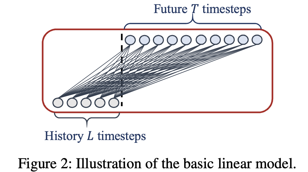
LTSF-Linear is a set of linear models.

• Linear: It is just a one-layer linear model, but it outperforms Transformers.
• NLinear: To boost the performance of Linear when there is a distribution shift in the dataset, NLinear first subtracts the input by the last value of the sequence. Then, the input goes through a linear layer, and the subtracted part is added back before making the final prediction. The subtraction and addition in NLinear are a simple normalization for the input sequence.
• DLinear: It is a combination of a Decomposition scheme used in Autoformer and FEDformer with linear layers. It first decomposes a raw data input into a trend component by a moving average kernel and a remainder (seasonal) component. Then, two one-layer linear layers are applied to each component and we sum up the two features to get the final prediction. By explicitly handling trend, DLinear enhances the performance of a vanilla linear when there is a clear trend in the data.

Although LTSF-Linear is simple, it has some compelling characteristics:

• An O(1) maximum signal traversing path length: The shorter the path, the better the dependencies are captured, making LTSF-Linear capable of capturing both short-range and long-range temporal relations.
• High-efficiency: As each branch has only one linear layer, it costs much lower memory and fewer parameters and has a faster inference speed than existing Transformers.
• Interpretability: After training, we can visualize weights to have some insights on the predicted values.
• Easy-to-use: LTSF-Linear can be obtained easily without tuning model hyper-parameters.

Comparison with Transformers

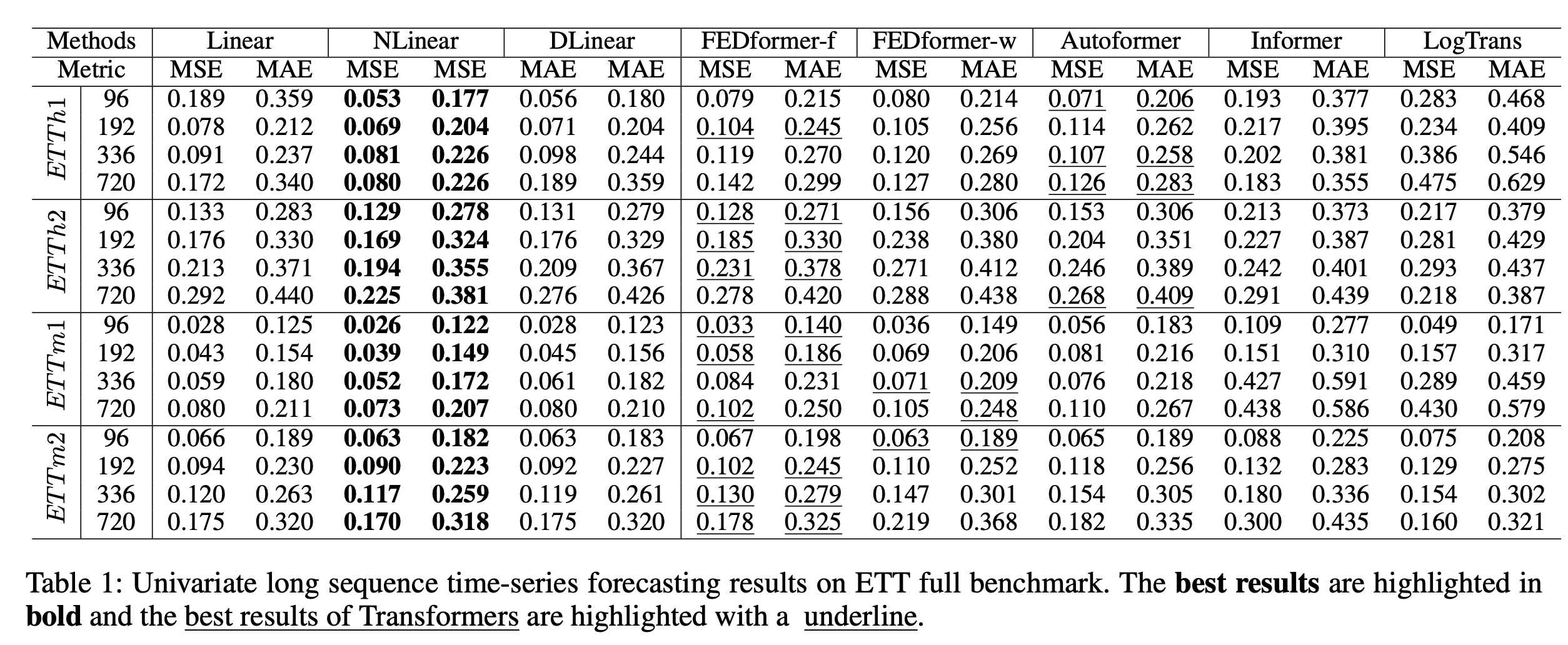
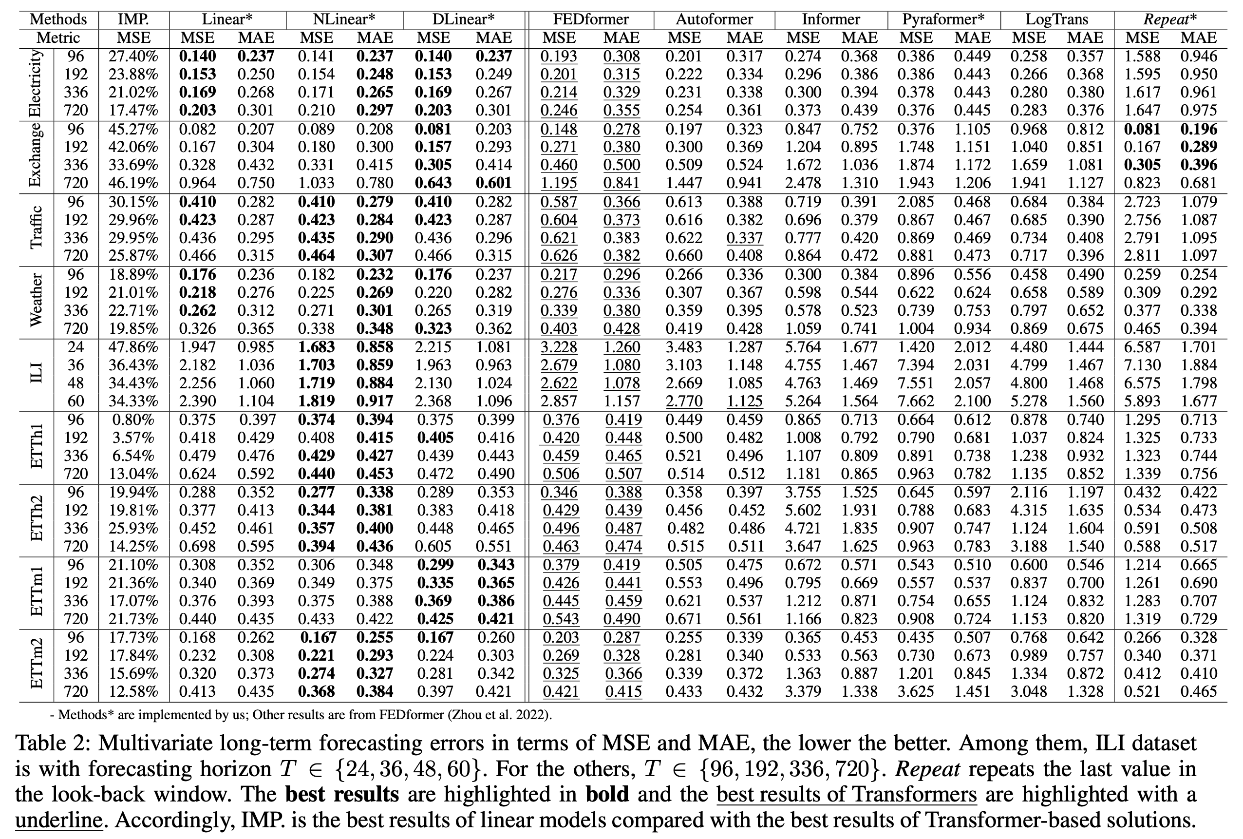
Univariate Forecasting: Multivariate Forecasting: LTSF-Linear outperforms all transformer-based methods by a large margin.

Efficiency

Comparison of method efficiency with Look-back window size 96 and Forecasting steps 720 on Electricity. MACs are the number of multiply-accumulate operations. We use DLinear for comparison, since it has the double cost in LTSF-Linear. The inference time averages 5 runs.

Getting Started

Environment Requirements

First, please make sure you have installed Conda. Then, our environment can be installed by:

conda create -n LTSF_Linear python=3.6.9
conda activate LTSF_Linear
pip install -r requirements.txt

Data Preparation

You can obtain all the nine benchmarks from Google Drive provided in Autoformer. All the datasets are well pre-processed and can be used easily.

mkdir dataset

Please put them in the ./dataset directory

Training Example

• In scripts/ , we provide the model implementation Dlinear/Autoformer/Informer/Transformer
• In FEDformer/scripts/, we provide the FEDformer implementation
• In Pyraformer/scripts/, we provide the Pyraformer implementation

For example:

To train the LTSF-Linear on Exchange-Rate dataset, you can use the scipt scripts/EXP-LongForecasting/Linear/exchange_rate.sh:

sh scripts/EXP-LongForecasting/Linear/exchange_rate.sh

It will start to train DLinear by default, the results will be shown in logs/LongForecasting. You can specify the name of the model in the script. (Linear, DLinear, NLinear)

All scripts about using LTSF-Linear on long forecasting task is in scripts/EXP-LongForecasting/Linear/, you can run them in a similar way. The default look-back window in scripts is 336, LTSF-Linear generally achieves better results with longer look-back window as dicussed in the paper.

Scripts about look-back window size and long forecasting of FEDformer and Pyraformer is in FEDformer/scripts and Pyraformer/scripts, respectively. To run them, you need to first cd FEDformer or cd Pyraformer. Then, you can use sh to run them in a similar way. Logs will store in logs/.

Each experiment in scripts/EXP-LongForecasting/Linear/ takes 5min-20min. For other Transformer scripts, since we put all related experiments in one script file, directly running them will take 8 hours-1 day. You can keep the experiments you interested in and comment out the others.

Weights Visualization

As shown in our paper, the weights of LTSF-Linear can reveal some charateristic of the data, i.e., the periodicity. As an example, we provide the weight visualization of DLinear in weight_plot.py. To run the visualization, you need to input the model path (model_name) of DLinear (the model directory in ./checkpoint by default). To obtain smooth and clear patterns, you can use the initialization we provided in the file of linear models.

Citing

If you find this repository useful for your work, please consider citing it as follows:

@inproceedings{Zeng2022AreTE,
  title={Are Transformers Effective for Time Series Forecasting?},
  author={Ailing Zeng and Muxi Chen and Lei Zhang and Qiang Xu},
  journal={Proceedings of the AAAI Conference on Artificial Intelligence},
  year={2023}
}

Please remember to cite all the datasets and compared methods if you use them in your experiments.