In this excercise, solely the visual input from three front-facing cameras in a simulator are used to predict the steering angle of the car-simulator. The model was trained on two tracks with varios direction changes and lane changes. Several data-augmentation techniques and CNN architectures where tested and applied in order to improve upon the training process. The resulting model performs well on both tracks, at 17mph on the mountain track and 25mph on the lake track.
End-to-End (E2E) learning through convolutional deep neural networks was shown recently to perform better then hand-crafted feature extraction, object detection, behavior inference and decision making in the autonomous vehicle domain [1]. This is attributed to the ability of deep CNNs to innately capture complex details of the scene and their relations. The resulting proposal is that the stream of a monocular vision sensor will be enough to make the car drive itself around complex terrains.
In this excercise a video stream of a car being driven in simulation around two tracks was recorded, a 'lake' track and a 'mountain' track, named track-1 and track-2 respectively.
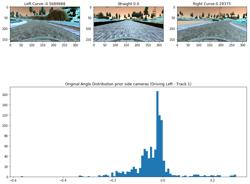
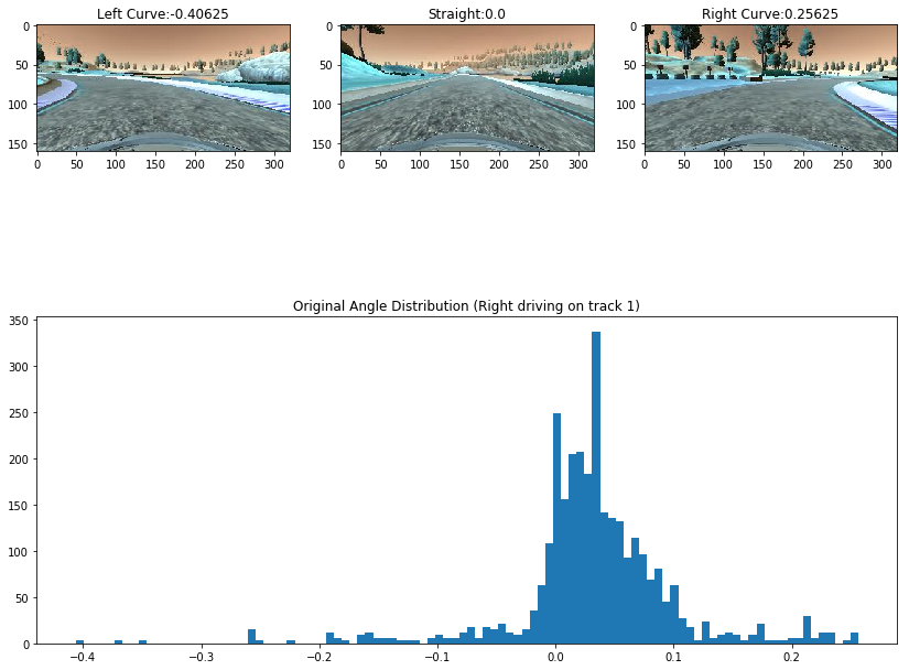
Track-1 is wide with interrupted lane markings, circumventing a lake. Although being at least twice as wide as the car in the simulator, the track proved to be difficult to be learned due to varios ligthning condition changes, texture changes on the road and surroundings, bridge crossings and interrupted lane markings.
Since going in a circle around the track will lead to predominance of turns in the direction of driving, the track was driven in both directions
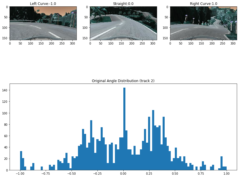
Track-2 is a two-lane mountain track with continuos markings but with a narrow lane-width. The horizon on this track is in some cases visible, but mostly not. Also the predominant background are dark-green steep hills, steep rocks and abysses. The terrain of track 2 is abbundant of steep climbs, drops and sharp turns.
The global lighting condition and scenery color distribution varies greatly between both tracks. To increase the ability of the network to generalize on both tracks, several pre-processing data augmentations where attempted.
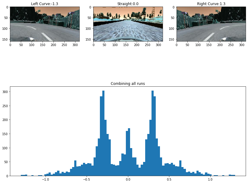
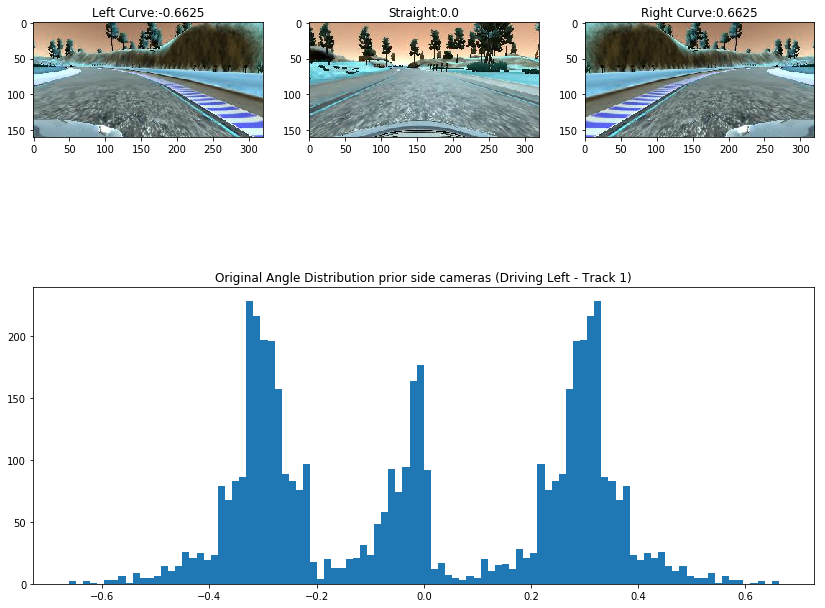
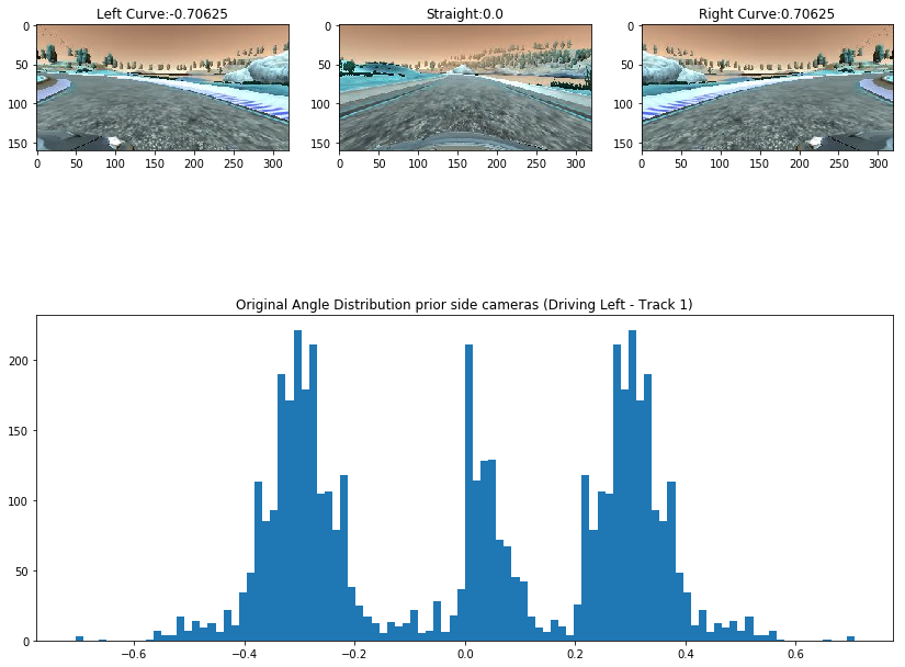
As can be seen, the steering angle distributions on track-1 depend on the direction being driven and are mostly concentrated around zero - i.e. around straight-line driving . Since it is necessary to train the car to make turns, as good as driving straight in a line, curved sections must be augmented and repeated.
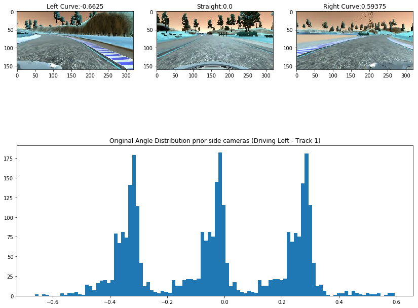
The simulator generates data from three camera locations, centre of car and left/right translated cameras. The left-right translation was assumed to impact the steering angle by a parametric threshold (0.25 < threshold < 0.35). This effectively tripples the dataset by solely adding images that simulate curves.
Sections of the data with a greater steering angle then a threshold (0.1 < threshold < 0.4) where flipped and their corresponding steering angles inverted.
Example: Track-1 Left driving flipped:
Example: Track-1 Right driving flipped:
As can be seen, image distributions now are approximately symmetrical mirror images of each other round the 0 axis.
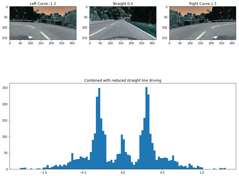
In order to improve upon the left-right driving differences, runs can be combined.
Since zero-angle images are still the most abbundant, their probability of occurrence was reduced to a parametric threshold (0.2 < threshold < 0.4)
Due to the large difference in backgrounds, methods for global lighting condition and background generalizations were seen as potentially benefitial.
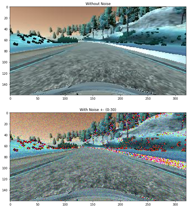
Images where augmented with random noise, through which each image pixel gets added or substracted a random value picked from a normal distribution with a parametric absolute maximum predefined.
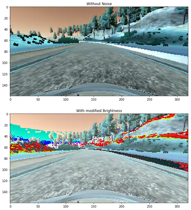
The global pixel values of images got added or subtracted a random value taken from a normal distribution with parametric absolute maximum and truncated to a uint8 compatible size.
Several different models where iterated through. However, the largest difficulty enountered was in regards to the available memory on the GPU that was used for the computations. It had a memory capacity of 2GB and that showed very fast the incapacity to work on medium to large convolutional nets.
The first and most crucial strategy to fit the data onto the device was to dynamically load-in data as required, rather then loading all of the data at once. This was achieved using a python generator.
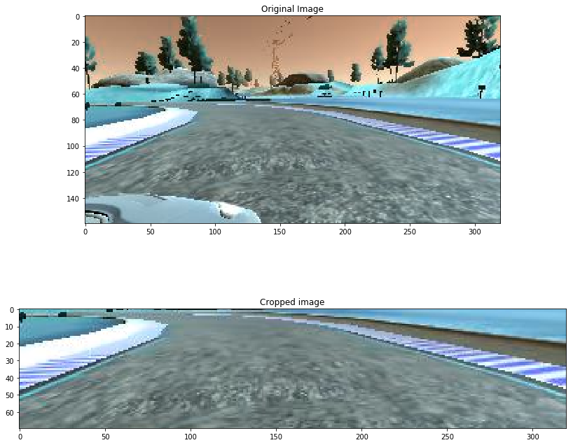
Each image consists of a road segment and background consisting of horizon, sky and terrain features. Since most of the usefull information is located on the bottom part of the image, the top part was cropped. Also, in the image, the complete vehicle is visible with a road segment behind it. This information is also redundant, hence it also can be cropped out. The crop ranges found are 65px from the top and 25px from the bottom.
Following ideas defined in [2], building the network was guided by attempting to gradually translate/convolute the spatial information to deep layers, eventually resulting in vector. This meant to minimize information loss in the first layers by lowering strides and increasing filter kernel footprint. It also meant to use average pooling at the start, rather then the more lossy max-pooling. Also, much of the design can be attributed to the limited memory size of the GPU device (2GB), on which the network was trained.
 Total params: 756,477
Trainable params: 756,477
Non-trainable params: 0
The first convolutional layer, after the image was read-in, normalized and cropped, was chosen to be with a relatively wide kernel (5,5) with a stride of (1,1) followed by an average pooling layer, in order to increase information propagation through the network.
The next couple of convolutional layers first gradually increase depth and reduce filter size then gradually decrease depth while further reducing filter size. Up until depth decrease, a max-pooling was used. Next no pooling was applied.
No dropouts were used in the convolutional layers as this showed to have reduced performance, which can be attributed to spatial-information loss.
Next, several fully connected layers were applied, seperated by dropout layers and all gradually decreasing their size to 1.
A mean-squared-error loss function and an Adam optimizer at default parameters, incl. learning rate (0.001).
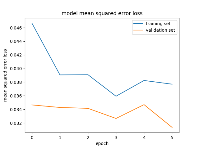
The training was performed in two-steps, a pre-training and training step. During pre-training only data from the second track was used for four epochs. During actual training all training sets were combined for four epochs, which achieved best performance.
After a number of attempts and parameter tweaking, a model was build that is able to drive the car accross both tracks for indefinite time.
The task was successfully completed.
[1] M. Bojarski, D. Del Testa, D. Dworakowski, B. Firner,B. Flepp, P. Goyal, L. D. Jackel, M. Monfort, U. Muller,J. Zhang, et al. End to end learning for self-driving cars, arXiv preprint arXiv:1604.07316, 2016
[2] Forrest N. Iandola and Song Han and Matthew W. Moskewicz and Khalid Ashraf and William J. Dally and Kurt Keutzer SqueezeNet: AlexNet-level accuracy with 50x fewer parameters and $<$0.5MB model size, 2016
