Term1-Project2: Traffic Sign Classifier
The primary goal of this project is to implement a CNN to recognize road traffic signs. In implementing the CNN, the emphasis is to understand the working principles & steps involved. Specifically,
- Exploring & visualizing the dataset
- Design, train and testing a model architecture
- Using the model to make prediction on new images
- Analyze the softmax probabilities of the new images
For this project we focus on the German road traffic signs. Specifically, we are using the dataset from The German Traffic Sign Recognition Benchmark (GTSRB).
The datasets constitutes of 43 classes and overall collection of ~52000 images. These images are further split into training, validation & test sets as depicted below
- training set = 34799
- validation set = 4410
- test set = 12630
Each sample is a 32x32 pixel image and the corresponding ground truth labels for each image is provided in csv file (; separated) with following structure
<img_number>;<label_number>
The labels are encoded into integers in the range of 0-42, and the corresponding mapping is provided in the signnames.csv
Example:
- Speed limit (20km/h)
- Speed limit (30km/h)
- Speed limit (50km/h)
- Speed limit (60km/h)
- Speed limit (70km/h)
- Speed limit (80km/h)
- End of speed limit (80km/h)
- Speed limit (100km/h)
- Speed limit (120km/h)
- No passing
- No passing for vehicles over 3.5 metric tons
...etc
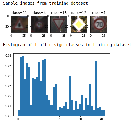
Here's a sample visualization of the training images and the histogram of the training set depicting the spread of traffic signs in the training set.
As shown in the image above, the CNN architecture consists of the following layers:
| Layer | Description | Params |
|---|---|---|
| Input | input samples | 32x32x1 |
| CONV 1 | convolution | filter_size=5x5, #filters=6, padding=0, stride=1, #bias=6 |
| RELU | activation | |
| POOL | sub sampling | kernel=2x2, stride=2, algo=max |
| CONV 2 | convolution | filter_size=5x5, #filters=16, padding=0, stride=1, #bias=16 |
| RELU | activation | |
| POOL | sub sampling | kernel=2x2, stride=2, algo=max |
| FC 1 | fully connected | input=5x5x16(400) output=120 |
| SOFTMAX | activation | |
| FC 2 | fully connected | input=120 output=84 |
| SOFTMAX | activation | |
| Output | output logits | input=84 output=43 |
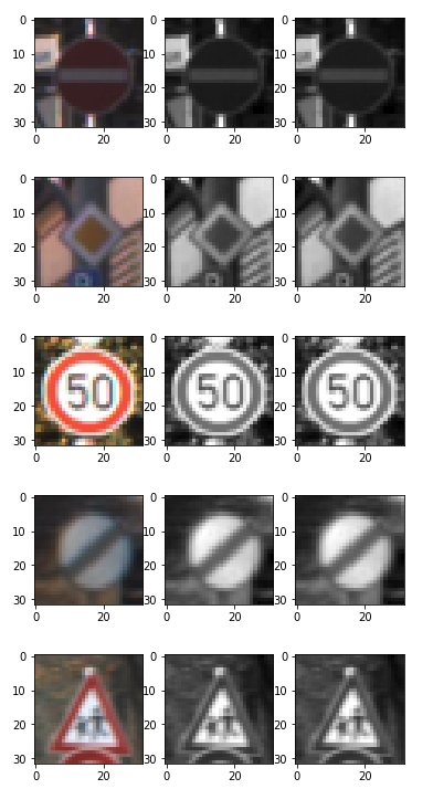
Grayscale Conversion As seen in the above design, the model expects the input samples to be in 32x32x1 format. We therefore convert our input samples from RGB (3 channels 32x32x3) to grascale (1 channel; 32x32x1).
Normalization Generally, it required that all the input data be on the same scale, which yields in faster convergence...etc benefits. While there are several methods to perform normalization, we perform a quick normalization on our input samples by subtracting & dividing each of our grayscale pixels by 28.
The image below shows sample images after pre-processing. column1 is the raw image sample, column2 is the grayscale and column3 is normalized.
The model was trained using the following components
- optimizer = Adam Optimizer
- batch size = 128
- epochs = 100
- learning rate = 0.001
- mean = 0
- std deviation = 0.1
I implement the famous LeNet CNN model for our traffic sign classifier. Although LeNet was originally designed for character recognition, we can use it for traffic sign classification as well since the core principle of this technique relies on recognizing patters/features in images rather than just matching a fixed set of key features as seen in other image matching solutions.
The following table highlights some of the experiments conducted
| Epochs | Batch size | learning rate | validation accuracy (%) | test accuracy (%) |
|---|---|---|---|---|
| 60 | 128 | 0.001 | 93.1 | 89.9 |
| 100 | 100 | 0.001 | 93.6 | 81 |
| 100 | 256 | 0.001 | 90.1 | 78.6 |
| 150 | 100 | 0.0001 | 91.8 | 68.9 |
| 100 | 128 | 0.001 | 94.9 | 92.6 |
| 150 | 128 | 0.001 | 95.5 | 93.3 |
Increasing the batch size beyond 128 didn't seem to show significant improvement. However, increasing the number of epochs resulted in higer accuracy in both validation & test set with learning rate at 0.001. Lowering the learning rate decreased accuracy. The optimal learning rate was see between 0.001-0.0009.
Therefore, the final model had the following results
- Epochs = 150, batch-size = 128, learning-rate = 0.001
- validation set accuracy = 95.5%
- test set accuracy = 93.3%
With the model finalized as described above, two sets of new images taken from the Internet was used for testing the model.
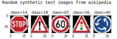
These traffic signs are digitally created traffic signs. since these kind of images represent the ideal scenario, I wanted to see how the model performed in such ideal sceanraios
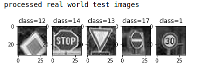
These traffic signs are also taken from the internet, but these are real world images with real world anomalies contained in the images (ex: oclussion, exposre & contrast, sheer change...etc). The models performace on these test image will depict the real world usage scenarios.
Synthetic test image = 100%
| Actual | predicted |
|---|---|
| Speed limit (60km/h) | Speed limit (60km/h) |
| stop | stop |
| General caution | General caution |
| Traffic signals | Traffic signals |
| Roundabout mandatory | Round about mandatory |
Real world test image = 83.3%
| Actual | prediction #1 | prediction #2 | prediction #3 | prediction #4 | prediction #5 |
|---|---|---|---|---|---|
| 3 | 29 (97.5) | 26 (2.3) | 17 (0.09) | 37 (0.05) | 28 (0.02) |
| 14 | 14 (100) | 1 (0) | 2 (0) | 33 (0) | 38 (0) |
| 18 | 13 (100) | 35 (0) | 9 (0) | 28 (0) | 12 (0) |
| 26 | 17 (100) | 33 (0) | 9 (0) | 34 (0) | 14 (0) |
| 40 | 38 (100) | 18 (0) | 34 (0) | 0 (0) | 25 (0) |
The visualizatoin with bar charts for these results is available in the notebook.
As expected, the synthetic data results in 100% accuracy since the images are extremely clear. Whereas in the real world images, the model only gave a 100% accurate result on only one sign (second row)
This solution & its results seen are from the direct adaptation of LeNet architecture for the traffic sign classification. Sermanet defines a modified version of LeNet which results in accuracy upto 99%. Key changes include
- changes to CNN architecture, where the results from CONV2 are also fed together into FC1
- chagnes in CNN architecture input layer to handle RGB color space.
- increasing training set by upsampling/adding morphed images for classes with less samples.


