Fast gradient-based optimization of resistance surfaces.
radish is an R package for maximum likelihood estimation of isolation-by-resistance models, where conductance is a function of spatial covariates, the observed data are genetic distances, and the likelihood of the "measurement process" is cheap to compute (e.g. regression of distance matrices, or generalized Wishart). It also provides fast computation of the gradient, Hessian matrix, and derivative-based leverage/influence measures. As currently implemented it is intended for moderate-sized problems (e.g. rasters with less than 1mil cells, where a sparse Cholesky decomposition of the graph Laplacian is feasible). Larger problems are possible (with sufficient memory), but slow.
To put this another way: if movement across a landscape is modeled as a continuous-time Markov process, and properties of this Markov process can be empirically observed (e.g. commute time, hitting time, occupancy time; or proxies thereof), then radish provides an algorithm to efficiently compute first- and second- order partial derivatives of a likelihood function with regard to entries of the infinitesimal generator of the Markov process. This is useful for fitting a parameterized Markov process -- where the entries of the infinitesimal generator depend on some low dimensional set of parameters -- to data, when the landscape is not trivially small. The algorithm implemented in radish is modular, so that any twice-differentiable function of a submatrix of the inverse infinitesimal generator could conceivably be used in the likelihood.
Slides from a recent workshop can be found here.
Requires corMLPE: devtools::install_github("nspope/corMLPE"). Other dependencies are available through CRAN. Install radish via devtools::install_github("nspope/radish").
This is a work-in-progress and the interface is still under development. Contact at nspope at utexas dot edu.
library(radish)
library(raster)

data(melip)

# scaling spatial covariates helps avoid numeric overflow
covariates <- raster::stack(list(altitude = raster::scale(melip.altitude),
                                 forestcover = raster::scale(melip.forestcover)))

plot(covariates[["altitude"]])
points(melip.coords, pch = 19)

surface <- conductance_surface(covariates, melip.coords, directions = 8)

fit_nnls <- radish(melip.Fst ~ forestcover + altitude, surface,
                   radish::loglinear_conductance, radish::leastsquares)
summary(fit_nnls)

# refit with with a different measurement model that models
# dependence among pairwise measurements (radish::mlpe)
fit_mlpe <- radish(melip.Fst ~ forestcover + altitude, surface,
                   radish::loglinear_conductance, radish::mlpe)
summary(fit_mlpe)

# visualisation:
plot(fitted(fit_mlpe, "distance"), melip.Fst, pch = 19,
     xlab = "Optimized resistance distance", ylab = "Fst")

# visualise estimated conductance surface and asymptotic confidence intervals
fitted_conductance <- conductance(surface, fit_mlpe, quantile = 0.95)

plot(fitted_conductance[["est"]],
     main = "Fitted conductance surface\n(forestcover + altitude)")
plot(fitted_conductance[["lower95"]],
     main = "Fitted conductance surface\n(lower 95% CI)")
plot(fitted_conductance[["upper95"]], main =
     "Fitted conductance surface\n(upper 95% CI)")

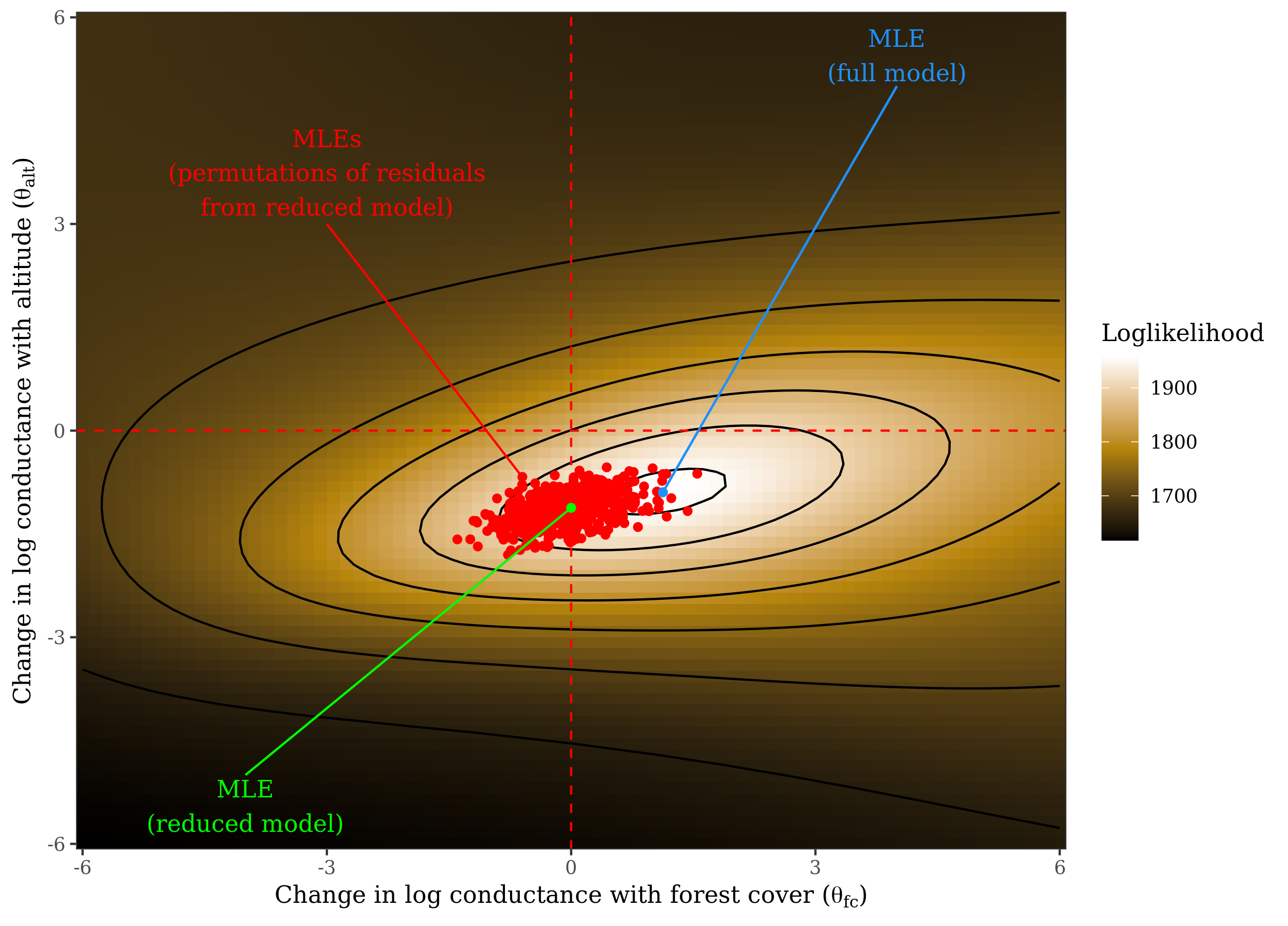
# visualise likelihood surface across grid (takes awhile)
theta <- as.matrix(expand.grid(forestcover=seq(-1,1,length.out=21),
                               altitude=seq(-1,1,length.out=21)))
grid <- radish_grid(theta, melip.Fst ~ forestcover + altitude, surface,
                    radish::loglinear_conductance, radish::mlpe)

library(ggplot2)
ggplot(data.frame(loglik=grid$loglik, grid$theta),
       aes(x=forestcover, y=altitude)) +
  geom_tile(aes(fill=loglik)) +
  geom_contour(aes(z=loglik), color="black") +
  annotate(geom = "point", colour = "red",
           x = coef(fit_mlpe)["forestcover"],
           y = coef(fit_mlpe)["altitude"]) +
  theme_bw() +
  xlab(expression(theta[altitude])) +
  ylab(expression(theta[forestcover]))

# calculate resistance distances across grid
distances <- radish_distance(theta, ~forestcover + altitude,
                             surface, radish::loglinear_conductance)

ibd <- which(theta[,1] == 0 & theta[,2] == 0)
plot(distances$distance[,,ibd], melip.Fst, pch = 19,
     xlab = "Null resistance distance (IBD)", ylab = "Fst")

# model selection:
# fit a reduced model without "forestcover" covariate, and compare to
# full model via a likelihood ratio test
fit_mlpe_reduced <- radish(melip.Fst ~ altitude, surface,
                           radish::loglinear_conductance, radish::mlpe)
anova(fit_mlpe, fit_mlpe_reduced)

# test for an interaction
fit_mlpe_interaction <- radish(melip.Fst ~ forestcover * altitude, surface,
                               radish::loglinear_conductance, radish::mlpe)
anova(fit_mlpe, fit_mlpe_interaction)

# test against null model of IBD
fit_mlpe_ibd <- radish(melip.Fst ~ 1, surface,
                       radish::loglinear_conductance, radish::mlpe)
anova(fit_mlpe, fit_mlpe_ibd)

# categorical covariates:
# rasters of categorical covariates must have an associated RAT, see ?raster::ratify
# the names of levels are taken from the VALUE column of the RAT, if it exists (otherwise,
# the integer codes are used)
forestcover_class <- cut(raster::values(melip.forestcover), breaks = c(0, 1/3, 1/6, 1))
melip.forestcover_cat <-
  raster::ratify(raster::setValues(melip.forestcover, as.numeric(forestcover_class)))

RAT <- levels(melip.forestcover_cat)[[1]]
RAT$VALUE <- levels(forestcover_class) #explicitly defines names in the RAT
levels(melip.forestcover_cat) <- RAT

covariates_cat <- raster::stack(list(forestcover = melip.forestcover_cat,
                                     altitude = melip.altitude))

surface_cat <- conductance_surface(covariates_cat, melip.coords, directions = 8)

fit_mlpe_cat <- radish(melip.Fst ~ forestcover + altitude, surface_cat,
                       radish::loglinear_conductance, radish::mlpe)

# contrast coding is the default for R, and for this conductance model
# the (non-identifiable) intercept is omitted (e.g. only relative
# differences in conductance among levels are identifiable from the data)
summary(fit_mlpe_cat)

# example of lower level interface:
# compute negative loglikelihood, gradient, Hessian for a given choice of
# of the conductance parameters theta, using a different measurement model
# (radish::generalized_wishart)
radish_algorithm(radish::loglinear_conductance(~forestcover + altitude, surface$x),
                 radish::generalized_wishart, surface,
                 pmax(melip.Fst, 0), nu = 1000, theta = c(-0.3, 0.3),
                 gradient = TRUE, hessian = TRUE)$hessian
# numerical verification (not run)
#numDeriv::hessian(function(x)
#     radish_algorithm(radish::loglinear_conductance(~forestcover + altitude, surface$x),
#                      radish::generalized_wishart, surface,
#                      pmax(melip.Fst, 0), nu = 1000, theta = x)$objective,
# c(-0.3, 0.3))In progress
