Example scripts for the weekly lessons of the faculty enrichment program 2022.
Overview: This readme includes detailed instructions for each week example exercise. An exercise usually consists of a simulation and an analyzer of simulation outputs. In some weeks, additional scripts exist to prepare simulation inputs or generate additional outputs and plots, or for model calibration as described in the instructions for the respective weeks. Weekly analyzer scripts already exists in the repository whereas the simulation scripts need to be copied over from Week 1 and further edited or newly created as instructed in following weeks.
Checking results: For each week suggested simulation scripts for comparison or help during the exercise are provided in the folder Solution_scripts. Also, at the end of the instructions results images and plots are included to compare against.
Prerequisites: Before running the weekly example scripts, please ensure that EMOD and dtk have been successfully installed and that the repository has been cloned to your local computer, ideally under /<.username>/Documents/faculty-enrich-2022-examples. It also needs dtk virtual environment loaded and assumes files are run from a working directory set to where the script is located. Before you start on an exercise, make sure that you have pulled or fetched the latest changes from the repository (see git-guides git-pull).
- Go to Week 1
- Go to Week 2
- Go to Week 3
- Go to Week 4
- Week 5: no technical track
- Go to Week 6
- Go to Week 7
- Go to Week 8
Table 1: Overview of main scripts used throughout the course
| Script | Description |
|---|---|
| analyzer_collection.py | collection of different analyzers used returning csv files |
| analyze_exampleSim_wX.py | the main analyzer script which changes each week (w1, w2,...w5) |
| generate_input_files.py | the default script for creating demographics and climate which needs to run only once or when substantial changes are made |
| plot_exampleSim_w4.py, plot_exampleSim_w4.R | plotting scripts outside of analyzer in python or R, introduced in Week 4 |
| run_exampleSim_wX.py | the main simulation script which will be expanded and modified throughout the lessons |
| simtools.ini | Configuration file for main directories required to run simulations (1 single file need in same directory where simulation or analyser script is run). Once paths have been defined, this file does not require any further editing. |
EMOD How To's:
- Update simtools.ini
- Define exp_name and identify expt_id
This week's exercise introduces the simplest version or running and analyzing a single simulation experiment in EMOD using the dtk infrastructure and python. Before running a simulation, one needs to check that all configurations and installations were successful and edit paths in simtools.ini file. The steps are 1) to run simulation and 2) to analyze simulation outputs. If that all works without any issues, the goal for week 1 has been reached!
Click to expand
- Adjust paths in
simtools.iniby replacing<USERNAME>with your username in path (5 locations) - Run simulation via
python run_exampleSim.py - Wait simulation to finish (~5 minutes)
- Note, when running locally, the console might return an psutil.AccessDenied text error, however the simulation can still successfully run and finish.
- If there are problems with running locally, you can peek into Week 6 on how to change
SetupParserto run on COMPS (requires login)!
- Go to the
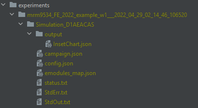
experiments/folder to notice the generated simulation experiment named ' username_FE_2022_example_w1___2022_04_29_02_14_46_106520' The last part after the '___' is the experiment id and changes with each simulation. - Update expt_id in
analyze_exampleSim_w1.pyLine 14 (copy number sequence after ___, also printed to console) - Run analyzer via
python analyze_exampleSim_w1.py - Inspect
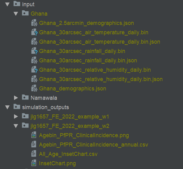
simulation_outputs/to see generated simulation results (csv file and plot) - Done!
Check results
Terminal output after running run_exampleSim.py 
Once finished 
Terminal output after running analyze_exampleSim_w1.py

Generated simulation output files
All_Age_Monthly_Cases.csv shows selected monitored malaria outcomes for the total population in the simulation
aggregated per month for the simulation duration, in this example 1 year.
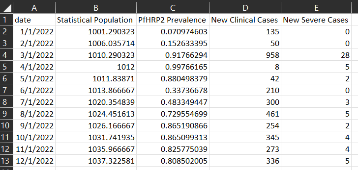
Generated plot
EMOD How To's:
- Update config parameters
- Create a demographics file
- Create climate files
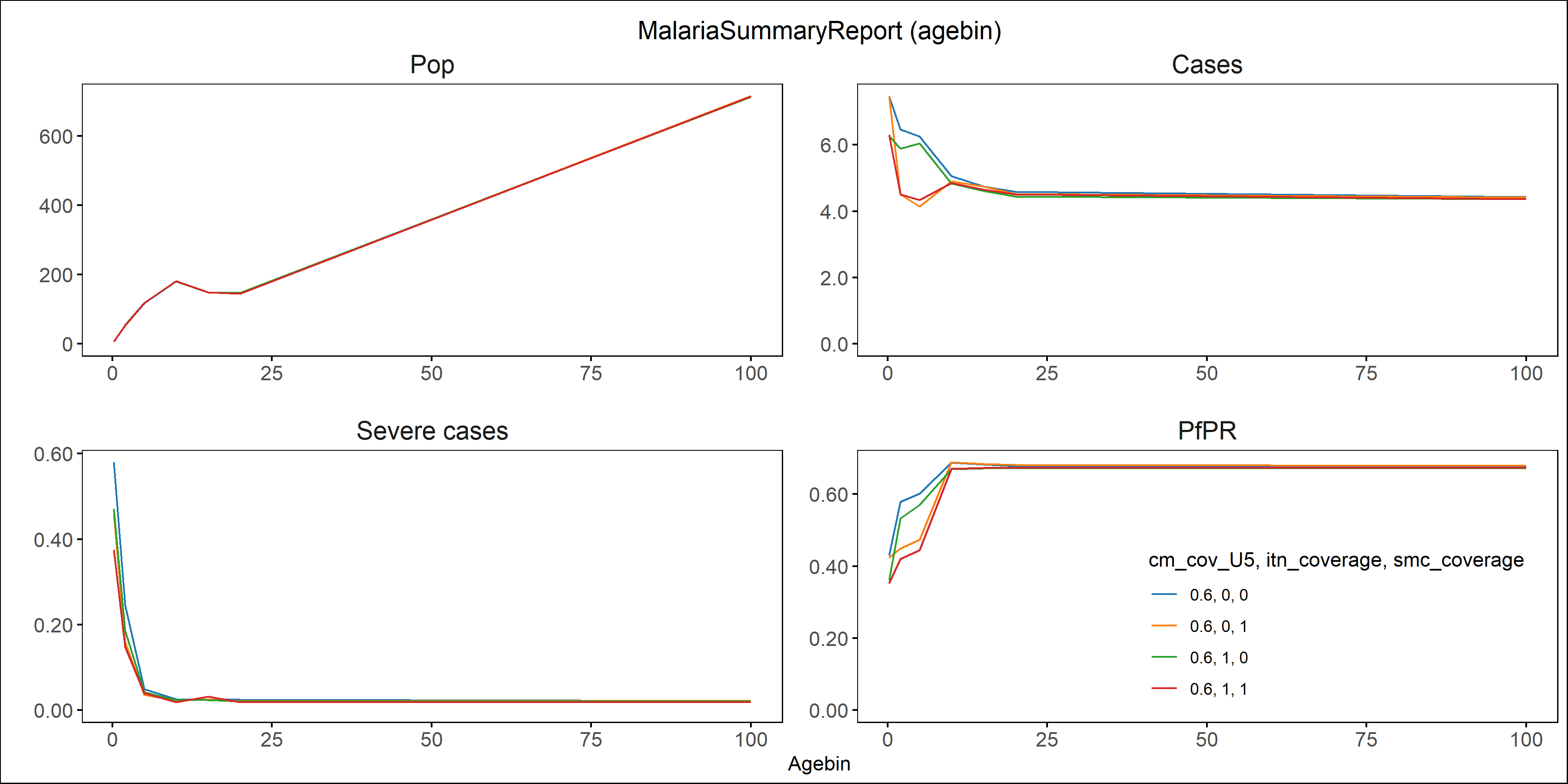
- Add summary reports ( annual)
- Set up multi-simulation experiments
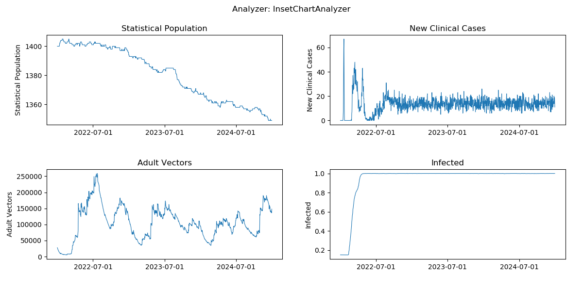
This week's exercise demonstrates how to create demographics and climate files and how to incorporate these into the simulation. The exercise further introduces how to modify config parameters (i.e. population size or simulation duration) and observe changes in simulation results based on the InsetChart.json model outputs.
Click here to expand
-
Create demographics and climate files via
python generate_input_files.py(requires access to COMPS for climate database : ask someone from NU team) -
Copy
run_exampleSim.pyand name itrun_exampleSim_w2.pyand in the script change exp_name tof'{user}_FE_2022_example_w2' -
Update default parameters in your simulation script (
run_exampleSim_w2.py):cb.update_params({ 'Demographics_Filenames': [os.path.join('Ghana', 'Ghana_2.5arcmin_demographics.json')], "Air_Temperature_Filename": os.path.join('Ghana', 'Ghana_30arcsec_air_temperature_daily.bin'), "Land_Temperature_Filename": os.path.join('Ghana', 'Ghana_30arcsec_air_temperature_daily.bin'), "Rainfall_Filename": os.path.join('Ghana', 'Ghana_30arcsec_rainfall_daily.bin'), "Relative_Humidity_Filename": os.path.join('Ghana', 'Ghana_30arcsec_relative_humidity_daily.bin'), "Age_Initialization_Distribution_Type": 'DISTRIBUTION_COMPLEX' })
-
Add custom reporter with annual summary for different age groups (see EMOD How To's) or suggested example below. Add the import statement at the top and the call to
add_summary_report()around line 26 (beforerun_sim_argsis defined):from malaria.reports.MalariaReport import add_summary_report add_summary_report(cb, start=1, interval=365, age_bins=[0.25, 2, 5, 10, 15, 20, 100, 120], description='Annual_Agebin')
-
Increase simulation duration from 1 to 3 years by modifying the initial call to DTKConfigBuilder:
years = 3
cb = DTKConfigBuilder.from_defaults('MALARIA_SIM', Simulation_Duration=years*365)
-
Run simulation as learned in week 1 and wait for simulation to finish (~5 minutes)
- Note, if there are problems with running locally, you can peek into Week 6 on how to
change
SetupParserto run on COMPS (requires login)!
- Note, if there are problems with running locally, you can peek into Week 6 on how to
change
-
Run analyzer script for Week 2
analyze_exampleSim_w2.py(don't forget to update expt_id!) -
Inspect
simulation_outputsand the generated plots- Optional: rerun analyzer with plot for week 1 and compare.
- Note that EMOD is a stochastic model and any changes at low population size and few repetitions might be at random and not necessarily due to the parameter change!
-
Run additional simulations with different durations, population sizes or for different agebins (Tip: change exp_name to keep track of your simulations)
# Example of how to change additional parameters from the config file
cb.update_params({
      'x_Base_Population': 1,
      'x_Birth': 1,
      'x_Temporary_Larval_Habitat': 1
  })
-
Again, inspect the simulation outputs and compare them against each other:
- How do the outcomes change?
- What do you recognize about running time?
Check results
Generated plot from InsetChart
Generated plot from annual summmary report
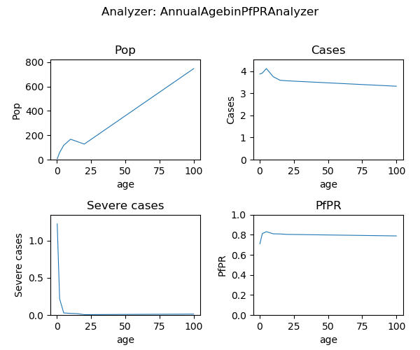
View suggested solution script for week 2
EMOD How To's:
- Case management
- Additional interventions
- Summary reports ( monthly)
- Event reporters
- Set up multi-simulation experiments
This week's exercise introduces how to implement the major malaria interventions in the EMOD simulation and is split into 2 parts:
- PART I - customization of the simulation, add interventions and reports
- PART II - multi-simulation experiment using ModBuilder
PART I, provides the parameterization or python code chunk for each of the main malaria interventions available in EMOD, and the exercise is to add these to the simulation script
together with proper 'reporting events' to be able to ensure that the intervention is successfully deployed in the simulation.
In addition, the ModBuilder is introduced in order to be able to run the same simulation multiple times, since EMOD is a stochastic model.
When simulating interventions, one might want to compare 'intervention' against 'no intervention', which can be achieved by expanding the ModBuilder to run multiple coverage values, or also other parameter values within a single experiments (PART II).
Click here to expand
-
Copy
run_exampleSim_w2.pyand name itrun_exampleSim_w3a.pyand in the script change exp_name tof'{user}_FE_2022_example_w3a' -
Add case management + 2 additional interventions of choice to your simulation script (
run_exampleSim_w3a.py). For each intervention, add the corresponding code chunk as well as module import into therun_exampleSim_w3a.py.- Suggested intervention code snippets:
-
add_health_seeking
 from malaria.interventions.health_seeking import add_health_seeking
 #Clinical cases
 add_health_seeking(cb, start_day=366,
                    targets=[{'trigger': 'NewClinicalCase', 'coverage': 0.7,
                              'agemin': 0, 'agemax': 5, 'seek': 1, 'rate': 0.3},
                             {'trigger': 'NewClinicalCase', 'coverage': 0.5,
                              'agemin': 5, 'agemax': 100, 'seek': 1, 'rate': 0.3}],
                    drug=['Artemether', 'Lumefantrine'])
 #Severe cases
 add_health_seeking(cb, start_day=366,
                    targets=[{'trigger': 'NewSevereCase', 'coverage': 0.49,
                     'seek': 1, 'rate': 0.5}],
            drug=['Artemether', 'Lumefantrine'],
            broadcast_event_name='Received_Severe_Treatment')
Note: two add_health_seeking events were added to allow tracking clinical and severe treatments separately
- First one uses default event 'Received_Treatment',
- second one uses 'Received_Severe_Treatment' by specifying
broadcast_event_name = 'Received_Severe_Treatment'
-
add_drug_campaign
 from malaria.interventions.malaria_drug_campaigns import add_drug_campaign

 add_drug_campaign(cb, campaign_type='SMC', drug_code='SPA',
                   coverage=0.8,
                   start_days=[366],
                   repetitions=4,
                   tsteps_btwn_repetitions=30,
                   target_group={'agemin': 0.25, 'agemax': 5},
                   receiving_drugs_event_name='Received_SMC')
Note: default event 'Received_Campaign_Drugs' has been changed by specifying
receiving_drugs_event_name ='Received_SMC' -
add_ITN
 from dtk.interventions.itn import add_ITN

 add_ITN(cb,
         start=366,  # starts on first day of second year
         coverage_by_ages=[
             {"coverage": 1, "min": 0, "max": 10},  # Highest coverage for 0-10 years old
             {"coverage": 0.75, "min": 10, "max": 50}, # 25% lower than for children for 10-50 years old
             {"coverage":  0.6, "min": 50, "max": 125} # 40% lower than for children for everyone else
         ],
         repetitions=5,  # ITN will be distributed 5 times
         tsteps_btwn_repetitions=365 * 3  # three years between ITN distributions
         )
Note: default event 'Received_ITN'. If desired to change this could be done by specifying
receiving_itn_event_name -
add_IRS
 from dtk.interventions.irs import add_IRS

 add_IRS(cb, start=366,
         coverage_by_ages=[{"coverage": 0.8, "min": 0, "max": 100}],
         killing_config={
             "class": "WaningEffectBoxExponential",
             "Box_Duration": 180,  # based on PMI data from Burkina
             "Decay_Time_Constant": 90,  # Sumishield from Benin
             "Initial_Effect": 0.7},
         )
Note: default event 'Received_IRS'. If desired to change this could be done by specifying
receiving_irs_event -
add_larvicides
 from dtk.interventions.novel_vector_control import add_larvicides

 add_larvicides(cb, start_day=366,
                habitat_target='CONSTANT',
                killing_initial=0.6,
                killing_decay=150
                )
-
add_vaccine
 from malaria.interventions.malaria_vaccine import add_vaccine

 add_vaccine(cb,
             vaccine_type='RTSS',
             vaccine_params={"Waning_Config":
                                 {"Initial_Effect": 0.8,
                                  "Decay_Time_Constant": 592.4066512,
                                  "class": 'WaningEffectExponential'}},
             start_days=[366],
             coverage=0.2,
             repetitions=1,
             tsteps_btwn_repetitions=-1,
             target_group={'agemin': 274, 'agemax': 275})  # children 9 months of age
Note: default event 'Received_Vaccine' and receiving_vaccine_event does not need to be specified in this case unless desired to change
-
- Suggested intervention code snippets:
-
To keep track of the campaign events in the simulations, add
event_listand expand as needed viaevent_list = event_list + [<new_event_name>]- Event
names:
'Received_Treatment', 'Received_Severe_Treatment','Received_ITN','Received_IRS', 'Received_SMC', 'Received_Vaccine'For example, if you added case management and ITNs, defineevent_listlike this:event_list = ['Received_Treatment', 'Received_ITN']
- Event
names:
-
Next, add an event reporter to monitor these events:
- Report_Event_Counter for aggregated event counts:
from malaria.reports.MalariaReport import add_event_counter_report

add_event_counter_report(cb, event_trigger_list=event_list, start=0, duration=10000)
- Report_Event_Recorder for individual events:
Note the Report_Event_Recorder output can get very large and usually is disabled for large interventions
cb.update_params({
   "Report_Event_Recorder": 1,
   "Report_Event_Recorder_Individual_Properties": [],
   "Report_Event_Recorder_Ignore_Events_In_List": 0,
   "Report_Event_Recorder_Events": event_list,
   'Custom_Individual_Events': event_list
})
- Report_Event_Counter for aggregated event counts:
-
Add
ModBuilderto allow running different stochastic seeds:from simtools.ModBuilder import ModBuilder, ModFn numseeds = 3 builder = ModBuilder.from_list([[ModFn(DTKConfigBuilder.set_param, 'Run_Number', x), ModFn(DTKConfigBuilder.set_param, 'Scenario', 'Basic') # optional ] for x in range(numseeds) ])
Adjust the
run_sim_argsblock to include the builder:run_sim_args = { 'exp_name': f'{user}_FE_2022_example_w3a', 'config_builder': cb, 'exp_builder' : builder }
-
Now, run the simulation and wait for it to finish (~5 minutes)
-
While simulations runs, look at the generated campaign file, does it include all interventions specified?
- The
campaign.jsonfile is located in your experiment simulation folder.
- The
-
Run analyzer script for Week 3 (
analyze_exampleSim_w3a.py)- Don't forget to update expt_id!
- And update
event_listin the analyzer to what you used inrun_exampleSim_w3a.py
-
Inspect the different results generated in
simulation_outputs.- Are all intervention events happening as expected?
- Parameters changes you can explore with further simulations:
- disable and enable interventions by changing coverage: be sure to change your experiment name if you run more experiments.
- does malaria transmission get interrupted if you set all to 1?
- age group receiving an intervention
- efficacy or start date of an intervention
- disable and enable interventions by changing coverage: be sure to change your experiment name if you run more experiments.
-
Extension: run another simulation to try out other interventions
- i.e. when using
add_ITN_age_seasoninstead ofadd_ITNit allows to track the custom events'Bednet_Got_New_One', 'Bednet_Using', 'Bednet_Discarded'.-
add_ITN_age_season
 from dtk.interventions.itn_age_season import add_ITN_age_season
 add_ITN_age_season(cb, start=366,
                    demographic_coverage=0.8,
                    killing_config={
                        "Initial_Effect": 0.520249973,  # LLIN Burkina
                        "Decay_Time_Constant": 1460,
                        "class": "WaningEffectExponential"},
                    blocking_config={
                        "Initial_Effect": 0.53,
                        "Decay_Time_Constant": 730,
                        "class": "WaningEffectExponential"},
                    discard_times={"Expiration_Period_Distribution": "DUAL_EXPONENTIAL_DISTRIBUTION",
                                   "Expiration_Period_Proportion_1": 0.9,
                                   "Expiration_Period_Mean_1": 365 * 1.7,  # Burkina 1.7
                                   "Expiration_Period_Mean_2": 3650},
                    age_dependence={'Times': [0, 100],
                                    'Values': [0.9, 0.9]},
                    duration=-1, birth_triggered=False
                    )
-
When the simulation is complete, try running the BednetUsageAnalyzer.
-
- i.e. when using
-
Extension: Try another analyzer such as the TransmissionReport.
-
Extension: Try adding ReportEventRecorder (see how-to's) and use the IndividualEventsAnalyzer to look at output.
Check results
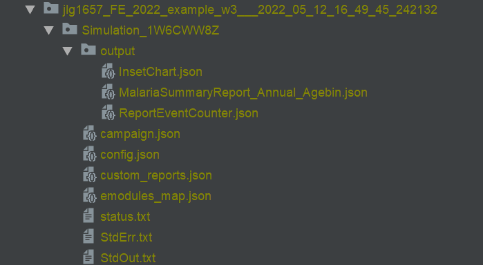
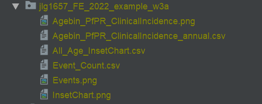
Raw output files in the experiment folder under outputs.
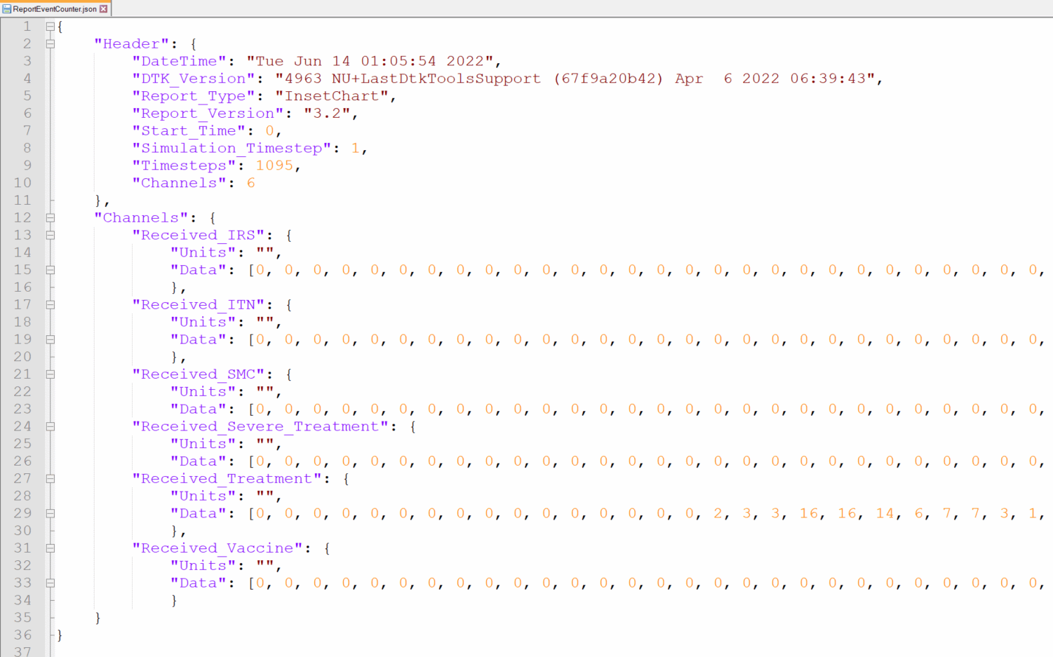
ReportEventCounter with campaign events, aggregated for total population. Most Interventions were set to start after
day 366, hence there are 365 zeros in the "Data": [0, 0, ...]
Tip: Notepad ++ offers helpful json plugins. Json files can also be viewed in Pycharm.
Generated results after running analyzer in simulation_outputs/<.exp_name>:
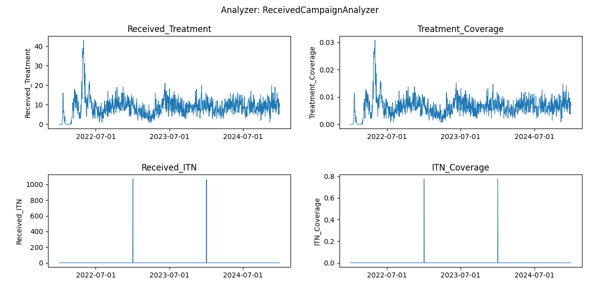
Aggregated event report
View suggested solution script for week 3 (a)
Click here to expand
-
Copy
run_exampleSim_w3a.pyand name itrun_exampleSim_w3b.pyand in the script change exp_name tof'{user}_FE_2022_example_w3b' -
ModBuilder can consume the same
add_x()intervention functions as used above in PART I, however it's often cleaner to wrap eachadd_x()into another function as shown below. For each intervention you wrap and use in the builder, make sure that it's not ALSO called directly usingadd_x().-
case_management
 def case_management(cb, cm_cov_U5, cm_cov_adults=0.5):
     add_health_seeking(cb, start_day=0,
                        targets=[{'trigger': 'NewClinicalCase', 'coverage': cm_cov_U5,
                                  'agemin': 0, 'agemax': 5, 'seek': 1, 'rate': 0.3},
                                 {'trigger': 'NewClinicalCase', 'coverage': cm_cov_adults,
                                  'agemin': 5, 'agemax': 100, 'seek': 1, 'rate': 0.3},
                                 {'trigger': 'NewSevereCase', 'coverage': 0.85,
                                  'agemin': 0, 'agemax': 100, 'seek': 1, 'rate': 0.5}],
                        drug=['Artemether', 'Lumefantrine'])

     return {'cm_cov_U5': cm_cov_U5,
             'cm_cov_adults': cm_cov_adults}
-
smc_intervention
 def smc_intervention(cb, coverage_level, day=366, cycles=4):
     add_drug_campaign(cb, campaign_type='SMC', drug_code='SPA',
                       coverage=coverage_level,
                       start_days=[day],
                       repetitions=cycles,
                       tsteps_btwn_repetitions=30,
                       target_group={'agemin': 0.25, 'agemax': 5},
                       receiving_drugs_event_name='Received_SMC')

     return {'smc_start': day,
             'smc_coverage': coverage_level}
-
itn_intervention
 def itn_intervention(cb, coverage_level, day=366):
     add_ITN(cb,
             start=day,  # starts on first day of second year
             coverage_by_ages=[
                 {"coverage": coverage_level, "min": 0, "max": 10},  # Highest coverage for 0-10 years old
                 {"coverage": coverage_level * 0.75, "min": 10, "max": 50},
                 # 25% lower than for children for 10-50 years old
                 {"coverage": coverage_level * 0.6, "min": 50, "max": 125}
                 # 40% lower than for children for everyone else
             ],
             repetitions=5,  # ITN will be distributed 5 times
             tsteps_btwn_repetitions=365 * 3  # three years between ITN distributions
             )
     return {'itn_start': day, 'itn_coverage': coverage_level}

event_list = event_list + ['Received_ITN']
 ### Or alternatiively
 def itn_intervention(cb, coverage_level, day=366):
     add_ITN_age_season(cb, start=day,
                        demographic_coverage=coverage_level,
                        killing_config={
                            "Initial_Effect": 0.520249973,  # LLIN Burkina
                            "Decay_Time_Constant": 1460,
                            "class": "WaningEffectExponential"},
                        blocking_config={
                            "Initial_Effect": 0.53,
                            "Decay_Time_Constant": 730,
                            "class": "WaningEffectExponential"},
                        discard_times={"Expiration_Period_Distribution": "DUAL_EXPONENTIAL_DISTRIBUTION",
                                       "Expiration_Period_Proportion_1": 0.9,
                                       "Expiration_Period_Mean_1": 365 * 1.7,  # Burkina 1.7
                                       "Expiration_Period_Mean_2": 3650},
                        age_dependence={'Times': [0, 100],
                                        'Values': [0.9, 0.9]},
                        duration=-1, birth_triggered=False
                        )

     return {'itn_start': day,
             'itn_coverage': coverage_level}

event_list = event_list + ['Bednet_Got_New_One', 'Bednet_Using', 'Bednet_Discarded']  # when using add_ITN_age_season
-
irs_intervention
 # IRS, start after 1 year - single campaign
 def irs_intervention(cb, coverage_level, day=366):
     add_IRS(cb, start=day,
             coverage_by_ages=[{"coverage": coverage_level, "min": 0, "max": 100}],
             killing_config={
                 "class": "WaningEffectBoxExponential",
                 "Box_Duration": 180,  # based on PMI data from Burkina
                 "Decay_Time_Constant": 90,  # Sumishield from Benin
                 "Initial_Effect": 0.7},
             )

     return {'irs_start': day,
             'irs_coverage': coverage_level}
-
rtss_intervention
 # malaria vaccine (RTS,S), no booster start after 1 year
 def rtss_intervention(cb, coverage_level, day=366, agemin=274, agemax=275, initial_efficacy=0.8):
     add_vaccine(cb,
                 vaccine_type='RTSS',
                 vaccine_params={"Waning_Config":
                                     {"Initial_Effect": initial_efficacy,
                                      "Decay_Time_Constant": 592.4066512,
                                      "class": 'WaningEffectExponential'}},
                 start_days=[day],
                 coverage=coverage_level,
                 repetitions=1,
                 tsteps_btwn_repetitions=-1,
                 target_group={'agemin': agemin, 'agemax': agemax})  # children 9 months of age

     return {'rtss_start': day,
             'rtss_coverage': coverage_level,
             'rtss_initial_effect': initial_efficacy}
-
-
Modify the
ModBuilderto allow running different parameter sweeps for intervention coverage using the functions newly added:builder = ModBuilder.from_list([[ModFn(case_management, cm_cov_U5), ModFn(smc_intervention, coverage_level=smc_cov), ModFn(rtss_intervention, coverage_level=rtss_cov), ModFn(itn_intervention, coverage_level=itn_cov), ModFn(irs_intervention, coverage_level=irs_cov), ModFn(DTKConfigBuilder.set_param, 'Run_Number', x) ] for cm_cov_U5 in [0.6] for smc_cov in [0, 1] for rtss_cov in [0] for itn_cov in [0] for irs_cov in [0] for x in range(numseeds) ])
-
Run simulations
- While waiting, check out the generated experiment folder, that now includes more subfolders for each of the
single simulations. Open two campaign files and compare, do you see any differences?
(Tip: Many text editors allow side by side comparison of two scripts, automatically highlighting differences)
- While waiting, check out the generated experiment folder, that now includes more subfolders for each of the
single simulations. Open two campaign files and compare, do you see any differences?
-
Open second analyzer script for Week 3 (
analyze_exampleSim_w3b.py) to update the exp_id as usual, but now also check that all the relevant sweep variables are included in sweep_variables and all the events of interest are included in event_list. The sweep_variables need to change according to theModBuilderand custom functions that return parameters, which uniquely define single simulations.## Example of sweep_variables in analyzer (customize to your simulation) sweep_variables = ['cm_cov_U5', 'smc_coverage', 'itn_coverage', 'irs_coverage', 'rtss_coverage', 'Run_Number']
-
Inspect
simulation_outputsand compare against outputs from the previous week. -
Change intervention parameters in the
ModBuilderand repeat the simulation process to become more familiar with the whole process.
Check results
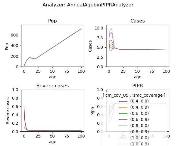
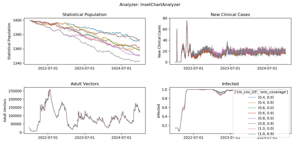
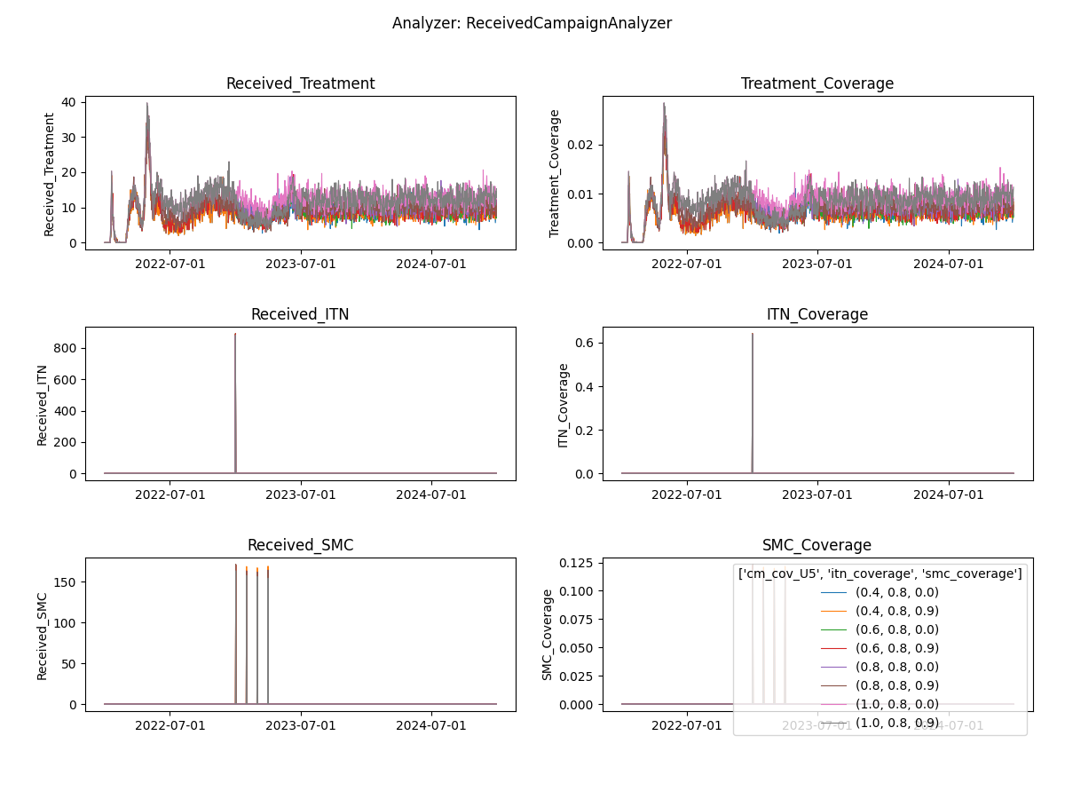
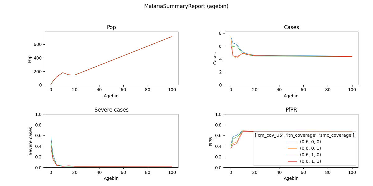
The generated result figures include separate lines. The Run_Numbers were aggregated using the mean and the intervention
coverage levels are used as additional grouping variables when aggregating simulation outputs. You may need to adjust the location of the legend if it's covering your plot!
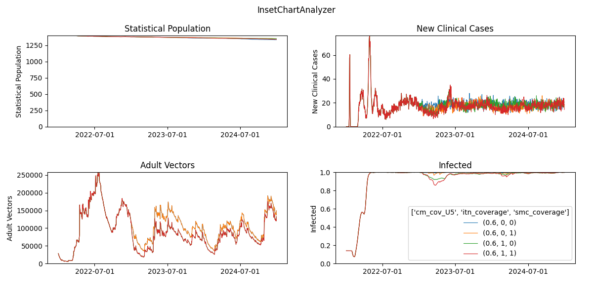
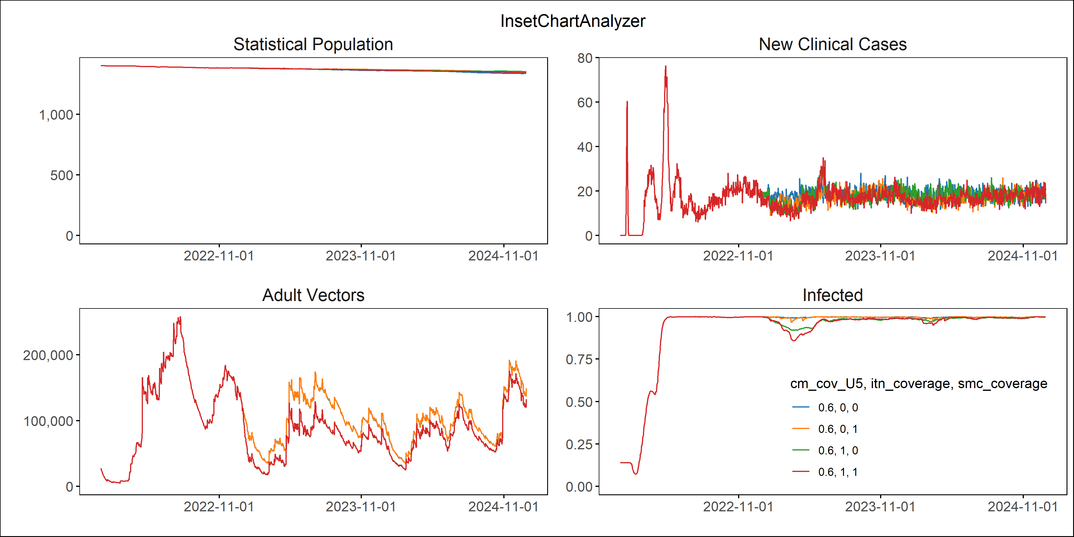
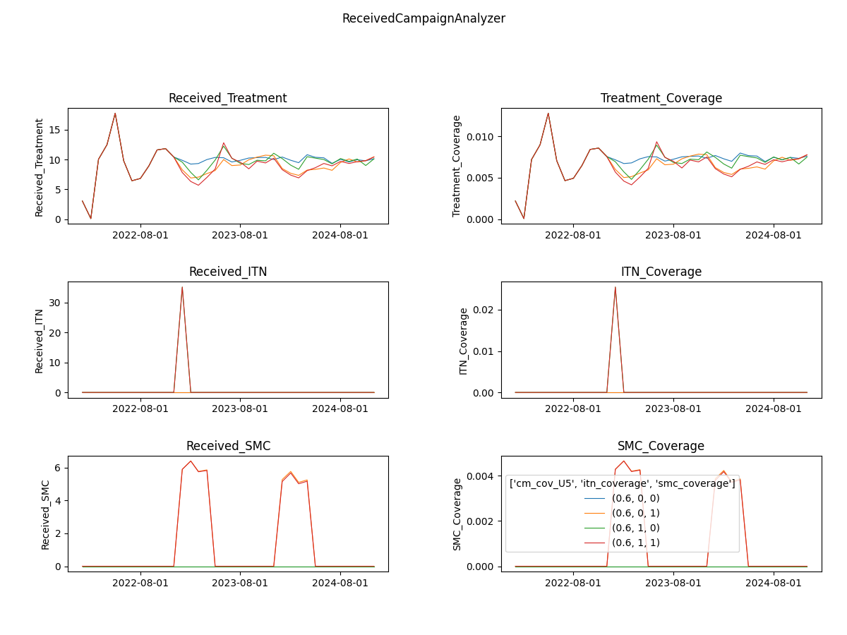
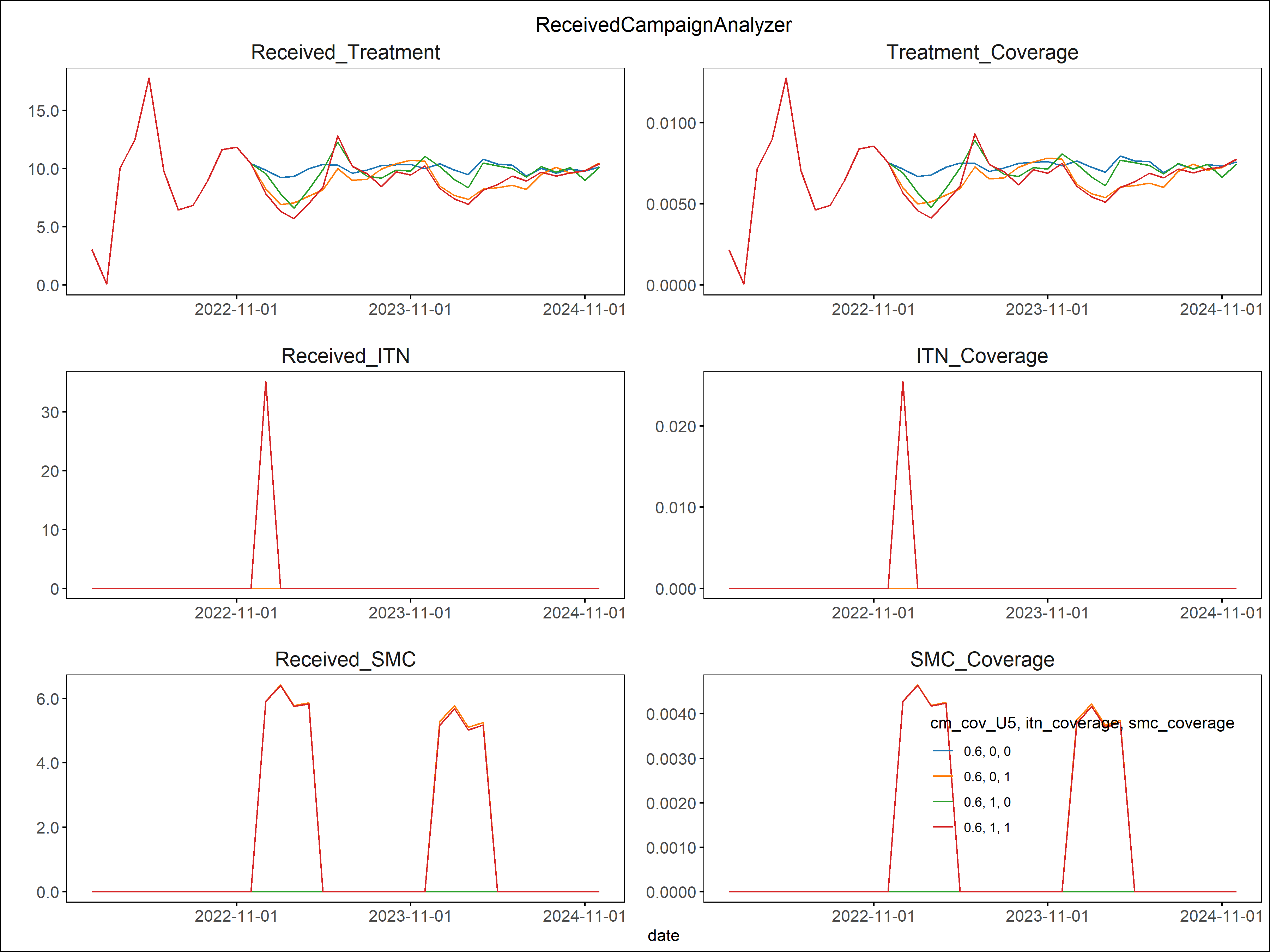
Examples with 4 levels of case management and 2 levels (off and on) of SMC:
Fig: Agebin_PfPR_ClinicalIncidence
Fig: All_Age_Monthly_Cases
Fig: Interventions distributed
Note, if too many parameters changed at once without clear labelling, the results can become difficult to interpret!
View suggested solution script for week 3 (b)
EMOD How To's:
This week's exercise focuses on the analyzer, i.e. the postprocessing of simulation outputs.
Specifically:
- analysing single simulation (already done Week 1-2)
- Multi-simulation experiment (introduced in Week 3, but more options for reporting available)
- Saving to csv (in previous weeks no csv was saved and plots automatically generated)
- Plotting in and outside of the analyzer using Python or R (this allows more flexibility and additional analysis after the simulation experiment finished)
The exercise is split into 2 parts: PART I adds more reporters for additional model output files to analyze and PART II provides examples of how to generate plots from the saved csv file from PART I.
Click here to expand
-
Copy
run_exampleSim_w3b.pyand name itrun_exampleSim_w4.pyand in the script change exp_name tof'{user}_FE_2022_example_w4' -
Cleanup your simulation script (
run_exampleSim_w4.py) of any unwanted interventions that were explored during the previous week- Adjust coverage levels in
ModBuilderto select/unselect interventions to include or change number of simulations to run (optional)
- Adjust coverage levels in
-
If not already there, enable or modify the individual-level event reporter as shown below. This example assumes there is case management for malaria in the simulation.
cb.update_params({
  'Report_Event_Recorder': 1,  # Enable generation of ReportEventRecorder.csv
  'Report_Event_Recorder_Ignore_Events_In_List': 0, # Logical indicating whether to include or exclude the events specified in the list
  'Report_Event_Recorder_Events': ['NewClinicalCase', 'Received_Treatment'], # List of events to include
  })
-
Add a new summary report with monthly monitoring for children under the age of 5 years only (keep min age 0.25)
for year in range(years):
  start_day = 365 + 365 * year
  sim_year = sim_start_year + year
  add_summary_report(cb, start=start_day, interval=30,
                     age_bins=[0.25, 5, 100],
                     description=f'Monthly_U5_{sim_year}')
-
Add
MalariaFilteredReportwhich is the same asInsetChartbut we can ask only to report on part of the simulation time (or just a subset of nodes, for spatial simulations).from malaria.reports.MalariaReport import add_filtered_report, add_event_counter_report add_filtered_report(cb, start=(years-1)*365, end=years * 365)
- Any analyzer script in analyzer_collection.py
that uses
InsetChart.jsoncan useReportMalariaFiltered.jsoninstead if you update theself.filenames=section.
- Any analyzer script in analyzer_collection.py
that uses
-
Run simulations
- While simulations are running, you may take a look at
analyze_exampleSim_w4.py, and correspondinganalyzer_collection.pyto explore the different Analyzer Classes used, no need to understand these in detail!
- While simulations are running, you may take a look at
-
Run the analyzer script
analyze_exampleSim_w4.py(remember to change exp_id :) )- This time, we didn't automatically generate plots! Now up to you to generate the plots you need.
-
Inspect
simulation_outputsand familiarize yourself with the csv files and match them to the analyzer + reports used in the simulation -
Run additional simulations and change the reports, for instance the agebins or reporting interval, and edit the analyzer accordingly (both
analyze_exampleSim_w4.py, and correspondinganalyzer_collection.py)!-
Change age group:
- Add summary report for children under the age of 10 (U10) in your simulation script.
- In the analyzer script, copy the analyzer MonthlyPfPRAnalyzerU5 and replace U5 with U10
- voilà a new analyzer for malaria outcomes aggregated for children under the age of 10 has been created!
- The principle of the MonthlyPfPRAnalyzers is the same for any age group as long as the indexing and number of agebins are matched correctly!
-
Change monitoring interval:
- Add summary report for weekly reporting in your simulation script.
- Note: In practice a monitoring intervals of either 365 or 30 days are easiest to interpret and collected data is also often per months or year. But in some occassions and also for exercise, weekly agebins might be of interest too (for shorter total simulation period).
-
Analyze additional outcome measures to look at (no new simulation needed)
- Look at the json file under
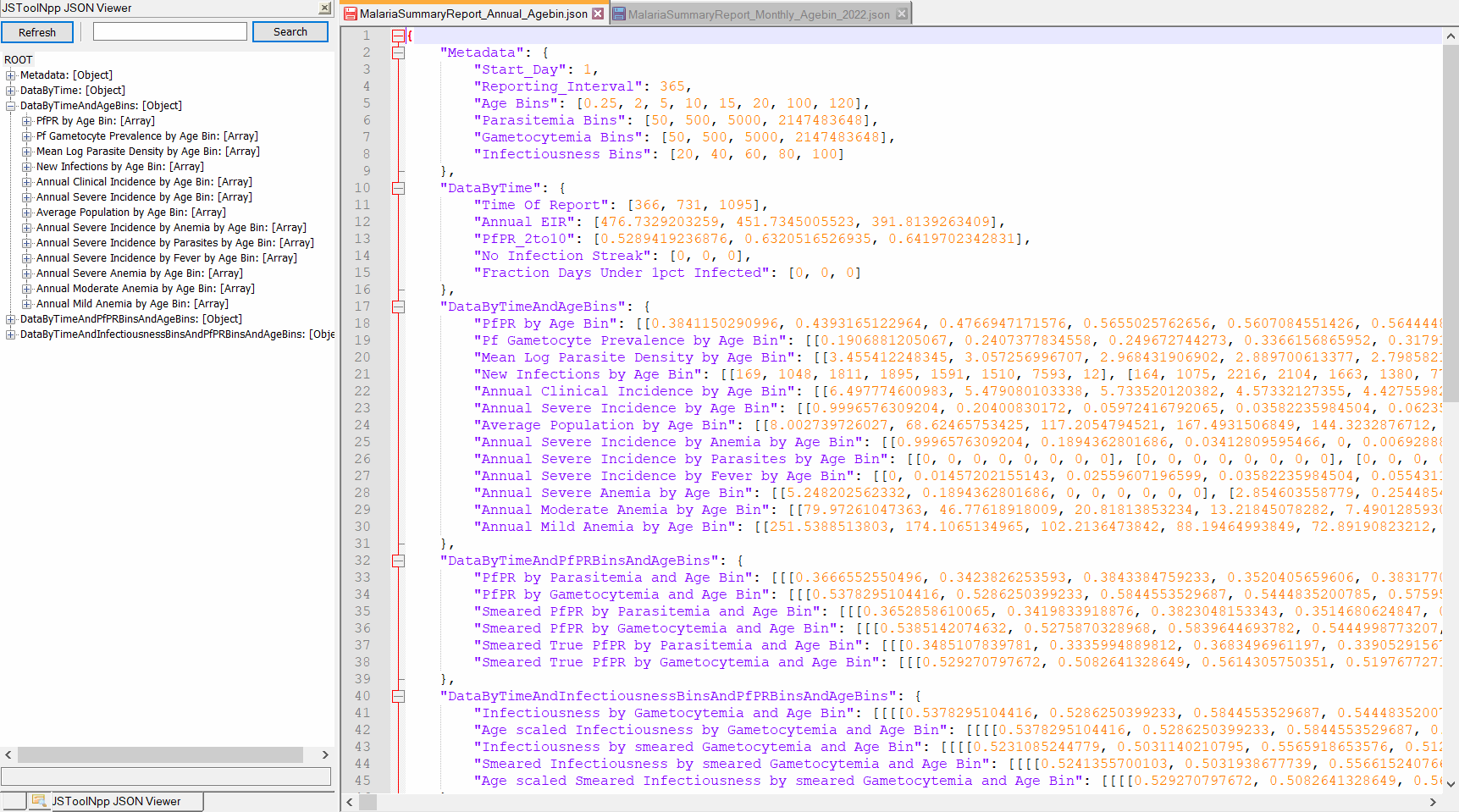
DataByTimeAndAgeBins(in COMPS or Notepadd++)- additional outcome examples 'New Infections by Age Bin', 'Annual Moderate Anemia by Age Bin', 'Mean Log Parasite Density by Age Bin'
- Add additional lines for new outcome measure, i.e. New Infections
py d = data[fname]['DataByTimeAndAgeBins']['New Infections by Age Bin'][:12] new_infect = [x[age] for x in d]py simdata = pd.DataFrame({'month': range(1, 13), 'PfPR': pfpr, 'Cases': clinical_cases, 'Severe cases': severe_cases, 'New infections': new_infect, ## newly added 'Pop': pop})
- Look at the json file under
-
-
Great! All the changes done demonstrate the flexibility of analyzers that can be highly customized to the user's and project needs. If you are interested to learn more about
reportersand how to analyze them, check out the EMOD How To's or IDM's EMOD documentation! -
Optional:
- Advanced: check the analyzer_collection.py for other analyzers that might be applicable to your simulation.
You also may have noticed that there are 2 analyzer commented out in
analyze_exampleSim_w4.py, you can try to uncomment them to enable them and rerun the analyzer. (Using comments is a convenient way to adjust which analyzers to run.) - It time: play around with json_explorer.py in Pycharm interactively to better understand reading in data from json selectively!
- Advanced: check the analyzer_collection.py for other analyzers that might be applicable to your simulation.
You also may have noticed that there are 2 analyzer commented out in
Check results
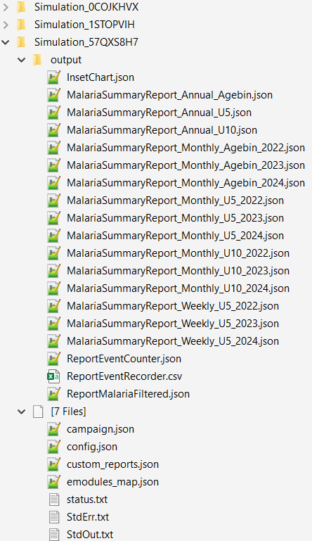
Example of EMOD generated simulation outputs
Example of a summary report json file, MalariaSummaryReport_Annual_Agebin.json
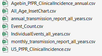
Example of simulation results, after running the analyzer (only csv files, see Part II for plots). The csv files that you should have:
- 'All_Age_InsetChart.csv' ,
- 'Agebin_PfPR_ClinicalIncidence_annual.csv' ,
- 'Event_Count.csv'
- 'U5_PfPR_ClinicalIncidence.csv' ## or more depending on additional summary reports for aggregated age
- 'annual_transmission_report_all_years.csv' ## (optional)
- 'IndividualEvents_all_years.csv' ## (optional)
View suggested solution scripts for week 4 simulation file , and edited analyzer file .
Click here to expand
- Check your csv files (see Part I) and make sure all required csv files were generated, optionally disable plots in the plotting script by commenting them out.
- Run plotting scripts either using Python or R:
- Python:
plot_exampleSim_w4.py - R:
plot_exampleSim_w4.R
- Python:
- Look at the figures more critically, anything you would like to change?
- Given the interventions implemented does the curves look as expected?
- Open the plotting script of your choice (python or R) and adjust axis titles, colors or even add your own plot!
- Note that the plots simply combine all sweep_variables in the legend. When having too many sweeps, the final output becomes difficult to interpret. These plots are good for diagnostic checks of correctness of experiment simulated, but not for presenting to others.
- Some suggested explorations _(no need to do all, some more meaningful than others ;)
- plot_inset_chart: per default plots selected channels over time per sweep_variables combination
- a) modify
channels_inset_chartto plot other channels (might need to adjust analyzer to write out more channels) - b) modify x axis to show date in different format and interval
- c) change color for no intervention (case management only) to black.
- d) add custom labels to sweep_variable combinations to have a better readable legend
- a) modify
- plot_summary_report:
- a) apply some of the changes done for plot_inset_chart to the summary report
- b) when you have added an additional age group analyzer, modify
Uageto plot results for the other age group
- plot_agebin_summary_report: per default aggregates all years to plot agebins on the x-axis, and has
multiple panels of defined channels (
channels_summary_report).- a) modify the figure to have agebin as color and unique_scen as panels, with time on the x-axis (annual or monthly summary report csv)
- b) modify the figure to have agebin as panels (facets) and time on the x-axis (annual or monthly summary report csv)
- plot_events:
- a) adjust y-axis to for coverage channels to show values as percentage
- b) set y-axis limits to have same y-axis for the left panels (number of individuals that received an intervention) and for the right panels (proportion of individuals that received an intervention)
- plot_inset_chart: per default plots selected channels over time per sweep_variables combination
EMOD How To's:
This week's exercise demonstrates the concept of serializing populations in simulations. Serialization allows us to run simulations, save them at a certain point in time, and simulate another campaign/scenario starting from the point we saved. We can run multiple simulations on the same population in series.
- We often use this process to save long initial simulations called "burnins", during which population immunity is established.
- We don't want to wait for this to run everytime, so we serialize the population at the end of the "burnin" and then run shorter simulations of interventions (also called "pickup" simulations).
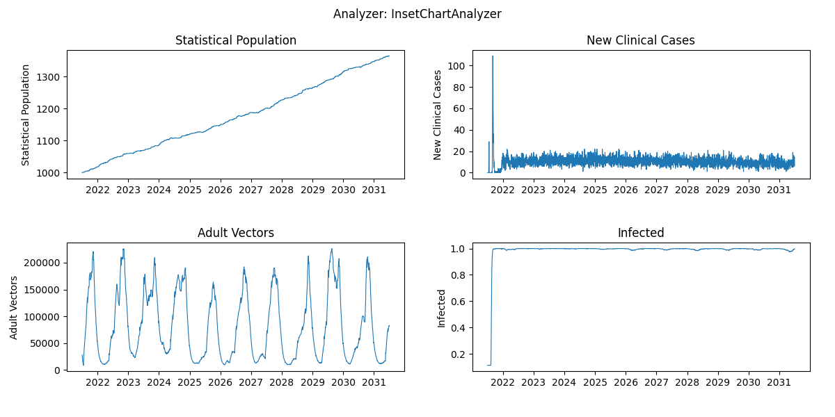
The exercise has three parts. In part 1 you will run and save a "burnin" simulation. In part 2 you will "pickup" this simulation and add antimalarial interventions. In part 3 you will repeat parts 1 & 2 using a longer "burnin" duration, and compare the results.
Click here to expand
- Create a new python script named 'run_exampleSim_w6a.py'
- Based on what you’ve learned from previous examples, add the basic code chunks needed to run a simulation, excluding interventions.
Check the details below for help and additional comments.
-
Import modules
 import os
 from dtk.utils.core.DTKConfigBuilder import DTKConfigBuilder
 from dtk.vector.species import set_species, set_larval_habitat
 from simtools.ExperimentManager.ExperimentManagerFactory import ExperimentManagerFactory
 from simtools.SetupParser import SetupParser
 from simtools.ModBuilder import ModBuilder, ModFn
-
SetupParser and SimulationDuration
- Run the simulation with 1 seed, and for 10 years. (For testing you might first run just 1 year). - Instead of `years`, define `serialize_years` and use 1 seed only - To keep track of the corresponding time in your experiment, you can include `sim_start_year = 2022 - serialize_years`
 SetupParser.default_block = 'HPC'
 numseeds = 1
 serialize_years = 10
 sim_start_year = 2022  - serialize_years

 cb = DTKConfigBuilder.from_defaults('MALARIA_SIM', Simulation_Duration=serialize_years * 365)
-
Demographics
 cb.update_params({
   'Demographics_Filenames': [os.path.join('Namawala', 'Namawala_single_node_demographics.json')],
   "Air_Temperature_Filename": os.path.join('Namawala', 'Namawala_single_node_air_temperature_daily.bin'),
   "Land_Temperature_Filename": os.path.join('Namawala', 'Namawala_single_node_land_temperature_daily.bin'),
   "Rainfall_Filename": os.path.join('Namawala', 'Namawala_single_node_rainfall_daily.bin'),
   "Relative_Humidity_Filename": os.path.join('Namawala', 'Namawala_single_node_relative_humidity_daily.bin')
 })
Note: You may either choose the default demographics for Namawala, or the one generated for Ghana.
-
Set vector species
 set_species(cb, ["arabiensis", "funestus", "gambiae"])
 set_larval_habitat(cb, {"arabiensis": {'TEMPORARY_RAINFALL': 7.5e9, 'CONSTANT': 1e7},
                         "funestus": {'WATER_VEGETATION': 4e8},
                         "gambiae": {'TEMPORARY_RAINFALL': 8.3e8, 'CONSTANT': 1e7}
                         })
-
Reporting
Reporting during the burnin simulation is optional, it depends on the simulation duration and what you want to track or to check. If not disabled InsetChart is automatically included, and can be plotted, alternatively one can disable the InsetChart and include an annual summary report to keep track of i.e. malaria metrics in an age group that is also plotted during the main simulation.
-
ModBuilder and run_sim_args
 builder = ModBuilder.from_list([[ModFn(DTKConfigBuilder.set_param, 'Run_Number', seed)]
                                 for seed in range(numseeds)
                                 ])

 user = os.getlogin()  # user initials
 run_sim_args = {
     'exp_name': f'{user}_FE_2022_example_w6a_50',
     'config_builder': cb,
     'exp_builder': builder
 }
-
exp_manager and run_simulations
if __name__ == "__main__":
    SetupParser.init()
    exp_manager = ExperimentManagerFactory.init()
    exp_manager.run_simulations(**run_sim_args)
    # Wait for the simulations to be done
    exp_manager.wait_for_finished(verbose=True)
    assert (exp_manager.succeeded())
 ```
</p>
</details>
-
- Now, to serialize the simulations so that you can “pick up” from them again later, add the code chunk below to update the serialization configuration parameters. (see Simple Burn-In in EMOD How To's). The section ideally would be placed before or after the other
cb.update_paramsin your script (i.e. after defining Demographics)-
Serialization
cb.update_params({
    'Serialization_Time_Steps': [365 * serialize_years],
    'Serialization_Type': 'TIMESTEP',
    'Serialized_Population_Writing_Type': 'TIMESTEP',
    'Serialized_Population_Reading_Type': 'NONE',
    'Serialization_Mask_Node_Write': 0,
    'Serialization_Precision': 'REDUCED'
})
Note: ‘serialize_years’ determines the duration of the simulation via
Simulation_Durationis also used to define theSerialization_Time_Steps
-
- If you have been testing with fewer years, run the simulation for 10 years (
serialize_years = 10) and update theexp_nameto reflect the duration, ex. 'burnin10'. - Run the analyzer
analyze_exampleSim_w6.pyto visualize the trend- Note, the analyzer script had been updated to allow running the same analyzer for PART I and PART II of the Week 6 examples,
therefore, ensure that
stepis set to 'burnin' and update theserialize_yearsto correspond to the number of years run in the burnin experiment (10).
- Note, the analyzer script had been updated to allow running the same analyzer for PART I and PART II of the Week 6 examples,
therefore, ensure that
- Optional:
- test out a longer burnin durations (ex. 50 years) and compare the time-series shown in the InsetChart plot.
Note: update the
exp_namei.e. add 'burnin50', to keep track of your simulation iterations
- test out a longer burnin durations (ex. 50 years) and compare the time-series shown in the InsetChart plot.
Note: update the
Click here to expand
-
Create a new simulation experiment
run_exampleSim_w6b.pythat will be used to run a simulation picking up from the 10-year burnin simulations you ran in PART I. -
To fill the script:
- copy the content from
run_exampleSim_w6a.pyinto the new script. - Add the following selected interventions and reporters for the future scenario simulation (see solution script):
- Case Management / Health-Seeking
- Starting on Day 0 of the pickup
- Treatment is with AL
- For NewClinicalCase:
- Coverage = 0.7 for children U5, 0.5 for all age 5+
- Seek = 1
- Rate = 0.3 (takes 3.33 days on average)
- For NewSevereCase:
- Coverage = 0.85 for all ages
- Seek = 1
- Rate = 0.5 (takes 2 days on average)
- ITNs
- Starting on Day 1 of Year 2 in the pickup
- Coverage of 0.6 for U5, 0.4 for ages 10-50 and 0.36 for ages 50+
- Distributed every 3 years of the pickup simulation
- Don't forget
- add 'Received_ITN' to the
event_list returnthe U5 coverage level
- add 'Received_ITN' to the
- Note that the start/end days for interventions and reports are relative to the beginning of the pick-up simulation - in other words, they re-start at zero.
- copy the content from
-
Add custom or new parameters that define the simulation and burnin duration as well as ID of the burnin experiment. Add these at the top of your new script after your import statements:
-
pickup_yearsto define your SimulationDuration (i.e. # of years post-burnin). This will replace theyearsorserialize_yearsthat you had previously in the script. -
pull_yearto define the year of the burn-in that serves as the start of the pick-up- Set equal to the value of
serialize_yearsinrun_exampleSim_w6a.py(either 10 or 50 years).
- Set equal to the value of
-
burnin_id = <exp_id>with the experiment_id from the burnin experiment you want to pick up from -
n_seedsto define the number of stochastic runs executed under each parameter setburnin_id = "b4f6741c-07da-ec11-a9f8-b88303911bc1" # UPDATE with burn-in experiment id pull_year = 10 # year of burn-in to pick-up from pickup_years = 5 # years of pick-up to run n_seeds = 3 # number of runs cb = DTKConfigBuilder.from_defaults('MALARIA_SIM', Simulation_Duration=pickup_years * 365)
-
-
retrieve output path from burnin experiment (see Picking up from Serialized Burn-in) in the EMOD How-To's.
-
import
retrieve_experimentfunction viafrom simtools.Utilities.Experiments import retrieve_experiment -
define
ser_dfexpt = retrieve_experiment(burnin_id) # Identifies the desired burn-in experiment # Loop through unique "tags" to distinguish between burn-in scenarios (ex. varied historical coverage levels) ser_df = pd.DataFrame([x.tags for x in expt.simulations]) ser_df["outpath"] = pd.Series([sim.get_path() for sim in expt.simulations])
-
-
Then, add/edit the serialization configuration parameters (so EMOD picks up this simulation from the one you ran in PART I).
```py cb.update_params({ 'Serialized_Population_Reading_Type': 'READ', 'Serialized_Population_Filenames': ['state-%05d.dtk' % (pull_year * 365)], 'Serialized_Population_Path': os.path.join(ser_df["outpath"][0], 'output'), # only use if having 1 single burnin 'Enable_Random_Generator_From_Serialized_Population': 0, 'Serialization_Mask_Node_Read': 0, 'Enable_Default_Reporting': 1, 'Disable_IP_Whitelist': 1 }) ``` _Notes: `pull_year` refers to the year of the burn-in to pickup from, usually the last year or the burnin. In this example, the simulation will pick-up on Jan 1 of year 10._-
Serialized_Population_Pathin the example above takes only the first scenario of the burnin simulation (ser_df["outpath"][0]). To match simulation tags and run number in pick up to those in burnin (when running multiple burnin scenarios in one experiment) thenSerialized_Population_Pathneeds to be defined in ModBuilder to allow sweeping through the scenarios of the burnin experiment (instead ofcb.update_params). You only need to do this if there is more than 1 burnin simulation in your experiment. You should only have one builder in your script - if you already have one for interventions, you would add the following code to it.builder = ModBuilder.from_list([ [ModFn(DTKConfigBuilder.set_param, 'Serialized_Population_Path', os.path.join(row['outpath'], 'output')), ModFn(DTKConfigBuilder.set_param, 'Run_Number', seed) ] for r, row in ser_df.iterrows() for seed in range(numseeds) ])
-
-
Run the experiment
-
Open the analyzer for week 6
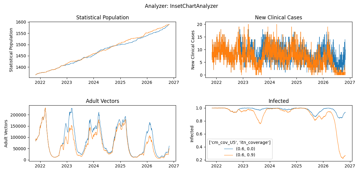
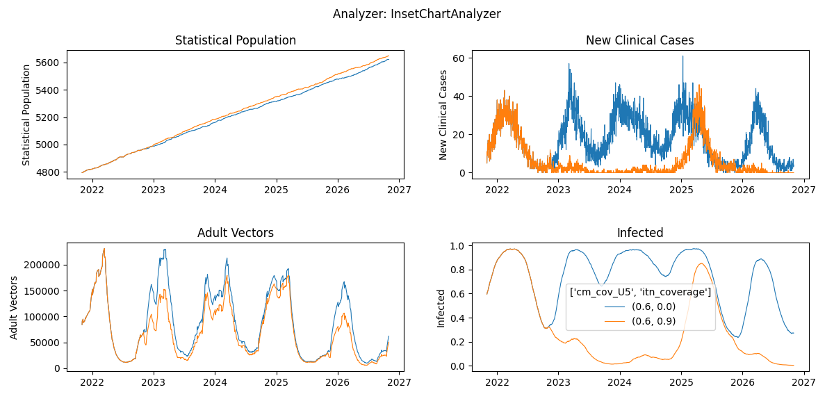
analyze_exampleSim_w6.pyand change some defaults commented out for PART I, then run the analyzer and check generated results.- update exp_name to 6b instead 6a
- update exp_id, as usual
- set
stepto 'pickup', this parameter has been added to allow running the same analyzer for both steps burnin and pickup - set
sweep_variablesto include any variables that differ between simulations within the experiment ['Run_Number' in this example].- You can see available variables as 'tags' if you run your simulations on COMPS.
-
Run
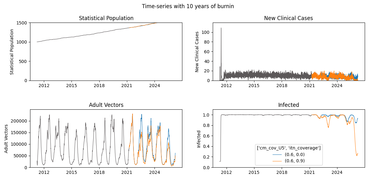
plot_exampleSim_w6.pyand notice the two time-series for both simulations combined in a single plot
Click here to expand
- If not already done, run
run_exampleSim_w6a.pywith a longer burn-in (50 years). - When it finishes running (may take a while), update the
burnin_idinrun_exampleSim_w6b.py - Before running the experiment, update the
exp_name(i.e. add 'burnin50'), to keep track of your simulation iterations Do not change anything else in the pickup simulation, to allow comparability across iterations picking up from different burnin durations. - Run the experiment
- Plot results using
plot_exampleSim_w6.pyor a custom plotter using summary report outcomes - Compare the plots between the experiments with 10 and 50 year burnins. Do you notice any difference?
Read Lesson Week 7 to understand the basics of sweeping and calibration, and the story behind this week's example.
Click here to expand
-
Modify
run_exampleBurnin_w6.pyscript with the following (You should duplicate and change the file name torun_exampleBurnin_w6.py.)- Change
serialize_yearsto 20 - Use
ModBuilderto run 5 simulations instead of 1 -
numseeds = 5 builder = ModBuilder.from_list([[ModFn(DTKConfigBuilder.set_param, 'Run_Number', x)] for x in range(numseeds)]) - Add the
ModBuilderobject intorun_sim_args - Modify
exp_namein therun_sim_argstof'{user}_FE_2022_example_w7a'
- Change
-
Run the burnin in COMPS
-
Modify
burnin_idinrun_examplePickup_w7.py, understand what is the script trying to achieve here. -
Run the 'pickup' in COMPS
-
Modify
expt_idinanalyze_exampleSim_w7.py -
Run the analyzer
-
Finally run the script
select_w7.py. This script calculate the average log-likelihood of eachitn_coveragebased on simulation output and produces some plots to visualize the parameter selection. -
Inspect the plot in the corresponding folder in
simulation_outputfolder. -
(Optional) Try running the whole procedure but using
Ghanainput files instead. The (fake) Ghana DHS data is located indata/w7_fake_DHS_Ghana.csv. What do you need to change so that selection of parameters is based on this dataset? -
(Optional) The choice of the
itn_coveragehere is based on 5 realizations which some may argue that the sample size is too small. Try to redo the exercise by increasing the number of realizations. Note that you need to decide if you want to rerun the burnin, or just increase the number of realizations in the pickup phase instead (What are the pros and cons of the two approaches?)
Check results
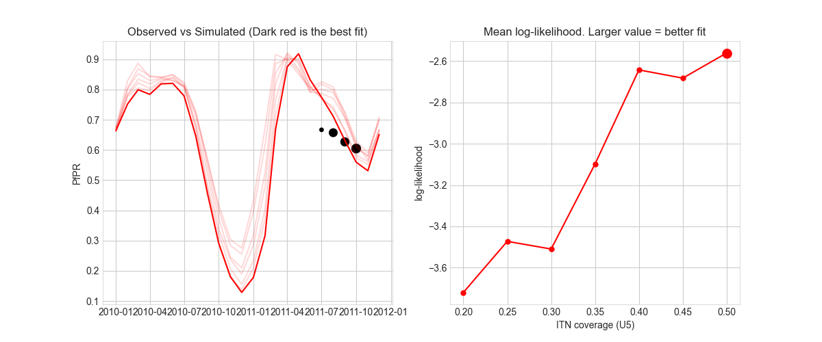
The log-likelihood of the itn_coverage would be printed out and look like this:
   itn_coverage        ll
0          0.20 -3.719067
1          0.25 -3.472211
2          0.30 -3.509376
3          0.35 -3.098715
4          0.40 -2.643516
5          0.45 -2.683272
6          0.50 -2.561883
And here is the plot out of select_w7.py script.
On the left is the observed data (size of bubble is proportionate to sample size) vs simulated mean PfPR trajectory.
On the right is the itn_coverage values and their corresponding log-likelihood.
EMOD How To's:
This week's example exercise introduces the concept and use case for individual properties. Individual properties allow to target specific groups of individuals by attaching a 'tag' or property to individuals in the simulation. These properties are completely customizable and for instance, they can be used to define intervention access, study enrollment, or drug response groups. It is also possible to have multiple individual properties.
- Individual properties for intervention access groups
- This example exercise uses individual properties to create 2 subgroups for intervention access: low access, high access.
- For simplicity, it is assumed that their relative size is equal (50% low access, 50% high access).
- Note that when deploying interventions at i.e. 80% coverage to the total population, the coverage for the subpopulations needs to be adjusted to reflect different population sizes, (covered in PART II).
In contrast to some other parameters, that can be easily switched on or off via cb.update_params,
individual properties need to be set up in the demographics file and also in the simulation script (to target campaign events or reports as needed).
- PART I shows how to modify the demographics file and asks to rerun a burnin similation (revisit week 6 for burnin), since demographics cannot be different in burnin and pick-up simulation.
- PART II shows a) how to target an intervention to subpopulations defined by individual properties, and b) how to get a summary report separately for the subpopulations. (Depending on the research question individual properties might only be needed for interventions and not for the reports, or vice versa, if not both.)
Click here to expand
- First, a new demographics file needs to be generated that defines individual properties.
- Modify
generate_input_files.pyas instructed below:-
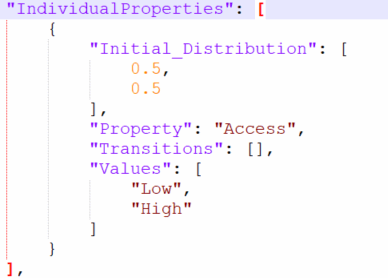
add a function that takes existing demographics json file and add individual properties to it in this example, we group individuals into a high and a low access group.
## Add Individual Properties (IPs)
def add_IPs(demo_fname):
    """Add Access IP"""
    IPs = [{'Property': 'Access',
            'Values': ['Low', 'High'],
            'Initial_Distribution': [0.5, 0.5],
            'Transitions': []}
           ]

    adf = pd.DataFrame({'Property': 'Access',
                        'Property_Value': ['Low', 'High'],
                        'Initial_Distribution': [0.5, 0.5]}
                       )
    adf['Property_Type'] = 'IP'
    adf['node'] = 1

    IP_demo_fname = os.path.join(demo_fname.replace('.json', '_wIP.json'))
    generate_demographics_properties(refdemo_fname=demo_fname,
                                     output_filename=IP_demo_fname,
                                     as_overlay=False,
                                     IPs=IPs,
                                     df=adf)
Instead of recreating the demographics and climate files, comment these out and add a call for the new
add_IPsfunction as shown below:inputs_path = os.path.join('./', 'input/Namawala')
demo_fname = os.path.join(inputs_path,'Namawala_single_node_demographics.json')
# generate_demographics(df, demo_fname)
# generate_climate(demo_fname)  # no need to generate a 2nd time
add_IPs(demo_fname)
-
- Run
python generate_input_files.pyto generate the new demographics json fileGhana_demographics_wIP.json, and inspect the file to check whether the IP's were successfully added.- Optional, do the same for the Ghana demographics
- Copy and rename both simulation scripts from week 7 to
run_exampleSim_w8a.pyandrun_exampleSim_w8b.py - In both simulation scripts:
- set
Disable_IP_Whitelistto 1 (if not already set at 1)cb.update_params({'Disable_IP_Whitelist' : 1})
- Update the demographics filename in
cb.update_params({ 'Demographics_Filenames': [os.path.join('Namawala', 'Namawala_single_node_demographics.json')],to read inNamawala_single_node_demographics_wIP.json - Change
exp_nameto week 8 to keep track of simulations + weeks
- set
- Submit burnin experiment to run
Click here to expand
Note: Having the IPs included in the demographics won't have any effect on the simulation if interventions or campaigns do not distinguish individuals by their properties.
-
Modify the
run_exampleSim_w8b.pyscript:- Add a helper function to re-calculate coverage depending on access group
- Modify the interventions (i.e.add_ITN) to customize coverage levels for low versus high access groups.
-
duplicate the
add_ITNwithin the defitn_interventionfunction -
add
ind_property_restrictionsto have one set of ITNs be distributed to the low, the other to the high access group. -
define two new parameters coverage_levels_low and coverage_levels_high
view modified itn_intervention
def itn_intervention(cb, coverage_level):
    ## Assume high access group = 0.5 of total population
    frac_high = 0.5
    if coverage_level > frac_high:
        coverage_level_high = 1
        coverage_level_low = (coverage_level - frac_high) / (1 - frac_high)
    else:
        coverage_level_low = 0
        coverage_level_high = coverage_level / frac_high

    add_ITN(cb,
            start=1,  # starts on first day of second year
            coverage_by_ages=[
                {"coverage": coverage_level_low, "min": 0, "max": 10},  # Highest coverage for 0-10 years old
                {"coverage": coverage_level_low * 0.75, "min": 10, "max": 50},
                # 25% lower than for children for 10-50 years old
                {"coverage": coverage_level_low * 0.6, "min": 50, "max": 125}
                # 40% lower than for children for everyone else
            ],
            repetitions=5,  # ITN will be distributed 5 times
            tsteps_btwn_repetitions=365 * 3,  # three years between ITN distributions
            ind_property_restrictions=[{'Access': 'Low'}]
            )

    add_ITN(cb,
            start=1,  # starts on first day of second year
            coverage_by_ages=[
                {"coverage": coverage_level_high, "min": 0, "max": 10},  # Highest coverage for 0-10 years old
                {"coverage": coverage_level_high * 0.75, "min": 10, "max": 50},
                # 25% lower than for children for 10-50 years old
                {"coverage": coverage_level_high * 0.6, "min": 50, "max": 125}
                # 40% lower than for children for everyone else
            ],
            repetitions=5,  # ITN will be distributed 5 times
            tsteps_btwn_repetitions=365 * 3,  # three years between ITN distributions
            ind_property_restrictions=[{'Access': 'High'}]
            )
    return {'itn_coverage': coverage_level}
-
add case management (see Week 3 for adding interventions)
view modified case_management function
def case_management(cb, cm_cov_U5=0.7, cm_cov_adults=0.5, cm_cov_severe=0.85):
    ## Assume high access group = 0.5 of total population
    frac_high = 0.5
    if cm_cov_U5 > frac_high:
        cm_cov_U5_high = 1
        cm_cov_U5_low = (cm_cov_U5 - frac_high) / (1 - frac_high)
    else:
        cm_cov_U5_low = 0
        cm_cov_U5_high = cm_cov_U5 / frac_high
    ## Optionally, depending on assumptions, do same for cm_cov_adults and cm_cov_severe

    add_health_seeking(cb, start_day=0,
                       targets=[{'trigger': 'NewClinicalCase', 'coverage': cm_cov_U5_low,
                                 'agemin': 0, 'agemax': 5, 'seek': 1, 'rate': 0.3},
                                {'trigger': 'NewClinicalCase', 'coverage': cm_cov_adults,
                                 'agemin': 5, 'agemax': 100, 'seek': 1, 'rate': 0.3},
                                {'trigger': 'NewSevereCase', 'coverage': cm_cov_severe,
                                 'agemin': 0, 'agemax': 100, 'seek': 1, 'rate': 0.5}],
                       drug=['Artemether', 'Lumefantrine'])

    add_health_seeking(cb, start_day=0,
                       targets=[{'trigger': 'NewClinicalCase', 'coverage': cm_cov_U5_high,
                                 'agemin': 0, 'agemax': 5, 'seek': 1, 'rate': 0.3},
                                {'trigger': 'NewClinicalCase', 'coverage': cm_cov_adults,
                                 'agemin': 5, 'agemax': 100, 'seek': 1, 'rate': 0.3},
                                {'trigger': 'NewSevereCase', 'coverage': cm_cov_severe,
                                 'agemin': 0, 'agemax': 100, 'seek': 1, 'rate': 0.5}],
                       drug=['Artemether', 'Lumefantrine'])

    return {'cm_cov_U5': cm_cov_U5,
            'cm_cov_adults': cm_cov_adults,
            'cm_cov_severe': cm_cov_severe}
-
For simplicity, set all intervention coverage levels >0.5 (due to the assumptions on coverage access made in this example)
-
Add additional reporters to be able to analyze results for both groups
 cb.update_params({
     'Report_Event_Recorder': 1,
     'Report_Event_Recorder_Individual_Properties': ['Access'],   ## add name of individual properties
     <...other report event parameter...>
 })
 sim_start_year = 2000 + pull_year # for convenience to read simulation times
 for i in range(pickup_years):
     add_summary_report(cb, start=1+365*i, interval=30,
                       duration_days=365,
                       age_bins=[0.25, 5, 120],
                       description=f'Monthly_U5_accesslow{sim_start_year+i}',
                       ipfilter = 'Access:Low')
     add_summary_report(cb, start=1+365*i, interval=30,
                       duration_days=365,
                       age_bins=[0.25, 5, 120],
                       description=f'Monthly_U5_accesshigh{sim_start_year+i}',
                       ipfilter = 'Access:High')
- Note: once we made sure it is doing what it is supposed to do, keeping reporters per group might not always be needed, depending on the research question
-
-
Once the burnin simulation finished, update exp_id in
run_exampleSim_w8b.py- Update ModBuilder to have only single coverage levels for the interventions included in your simulation (otherwise result plots will look messy)
-
Run the pickup experiment (
run_exampleSim_w8b.py) -
Run the analyzer script for Week 8
analyze_exampleSim_w8.py -
Inspect results, the generated plots as well as IndividualEvents
-
Options for further exploration:
- Rerun burnin + pickup simulation with different ratio between low and high access group
-
Think about what other individual properties would be useful and how these could be implemented.
Check results
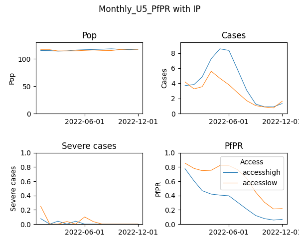
Simulation outputs showing summary reports per Access group used as example for individual properties
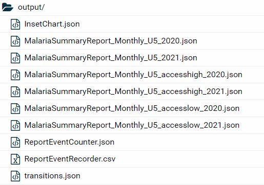
Plot of aggregated malaria burden over time per Access group
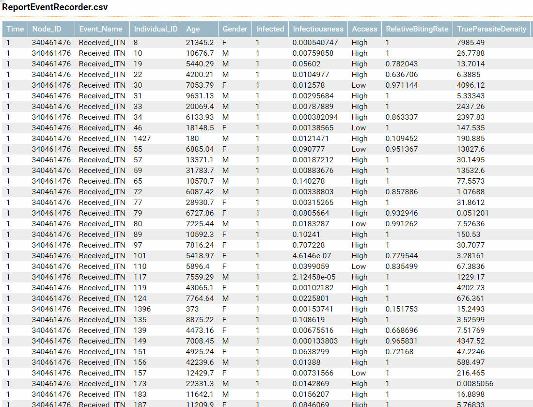
Report Event Recorder including individual properties
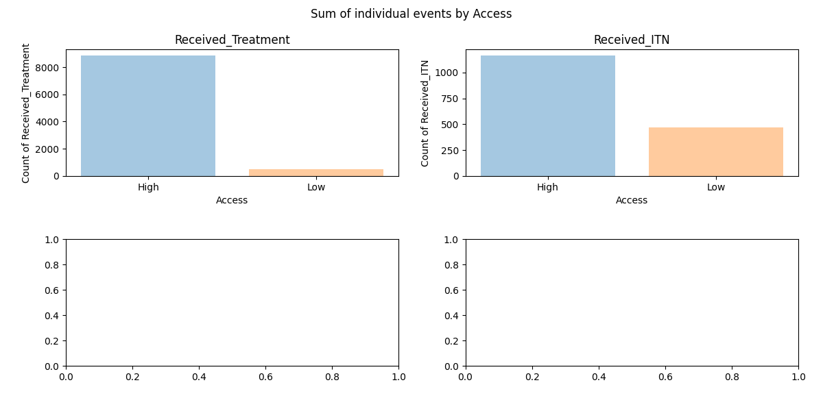
Simple barplot showing sum of individuals per group that received an intervention
You reached the end of the example lessons. Please check on the website for additional content for the following weeks.
