Educational simulations for understanding the MRI signal. This project is created for OHBM Brainhack 2024. The main goal is to create single script simulations that builds up an understanding of the MRI signal step by step. Fundamental papers, and equations will be linked. The long term goal of this project is to build this repository as an educational resource to teach MRI basics. An important source of inspiration for this project is https://www.youtube.com/c/3blue1brown .
| Package | Tested version |
|---|---|
| matplotlib | 3.1.1 |
| NumPy | 1.22.0 |
Clone this repository, navigate to the folder, and execute in your terminal:
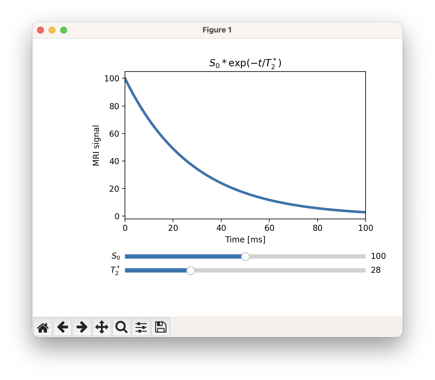
python 01_t2starsim_v1.py
If everything went well, you should be able to see and interactive figure as show below:

- Reading 1: [A very good starting point] Hagberg, G., Tuzzi, E., 2014. Phase Variations in fMRI Time Series Analysis: Friend or Foe?, in: Advanced Brain Neuroimaging Topics in Health and Disease - Methods and Applications. InTech. https://doi.org/10.5772/58275 We are going to reconvene at 15:00 to discuss Hagber, Tuzzi 2014 equations 2 and 3
- Task 1: After running
python 01_t2starsim_v1.pyand playing around with the parameters, implement Hagberg, Tuzzi 2014 Equation 3 (T1 relaxation). - Task 3: Write a new script where the users enters an echo time (e.g. 40 ms) and a percent signal change (e.g. 5 %) to compute the "required T2* change" to give rise to that percent signal change at the chosen echo time.
- Reading 2 : Understand Equation 1 of Uludag, K., Müller-Bierl, B., Ugurbil, K., 2009. An integrative model for neuronal activity-induced signal changes for gradient and spin echo functional imaging. NeuroImage 48, 150–65. https://doi.org/10.1016/j.neuroimage.2009.05.051 . Particularly, familiarize yourself with intravascular and extravascular components of the fMRI signal.
- Task 3: Please look at and run 02_T2starsim_v2.py and conteplate how it relates to Uludag et al. 2009 Equation 1.
- Reading 3: Sections 3.1 and 3.2 from Hagberg, G., Tuzzi, E., 2014. Phase Variations in fMRI Time Series Analysis: Friend or Foe?, in: Advanced Brain Neuroimaging Topics in Health and Disease - Methods and Applications. InTech. https://doi.org/10.5772/58275
- Task 3: Once you are done reading, run
03_generate_complex_numbers.pyprogram and contemplate. - Reading 4: See Figure 1 and 2 from: Gudbjartsson, H., Patz, S., 1995. The rician distribution of noisy mri data. Magnetic Resonance in Med 34, 910–914. https://doi.org/10.1002/mrm.1910340618 . Particularly, think about and compare how the statistical properties of magnitiude and phase signal change across low and high signal to noise ratio (SNR) regimes.
- Reading 5: Understand Equation 10 from Section 3.3 (you can avoid later parts of the section): from Hagberg, G., Tuzzi, E., 2014. Phase Variations in fMRI Time Series Analysis: Friend or Foe?, in: Advanced Brain Neuroimaging Topics in Health and Disease - Methods and Applications. InTech. https://doi.org/10.5772/58275
- Task 4: Run
04_boxerman1995_interactive.pyand contemplate the similarities or differences to Equation 10 from Hagberg, Tuzzi, 2014. Then, compare what you see to Figure 7 of the same article. - Reading 5: Understand Figure 1 and 2 from: Vu, A.T., Gallant, J.L., 2015. Using a novel source-localized phase regressor technique for evaluation of the vascular contribution to semantic category area localization in BOLD fMRI. Frontiers in Neuroscience 9, 1–13. https://doi.org/10.3389/fnins.2015.00411
- Reading 6: Now lets go back to the beginning of fMRI by having a look at Figure 4 and Equation 1 from: Ogawa, S., Lee, T., Nayak, A.S., Glynn, P., 1990. Oxygenation‐sensitive contrast in magnetic resonance image of rodent brain at high magnetic fields. Magnetic Resonance in Med 14, 68–78. https://doi.org/10.1002/mrm.1910140108
- Reading 7: Once you had a look at Figure 1 and Equation 1 from the Reading 6, switch to Figure 1 and 2 from: Menon, R.S., 2002. Postacquisition suppression of large‐vessel BOLD signals in high‐resolution fMRI. Magnetic Resonance in Med 47, 1–9. https://doi.org/10.1002/mrm.10041 . These figures and the text referring to these figures will elucidate further on the coupling between phase and magnitude fMRI signal, as well as connecting spin echo and gradient echo concepts.
- Reading 8: If you are struggling to understand or imagine the argument of Menon 2002 Figure 2, please look at the Figure 4 from: Hoogenraad, F.G.C., Reichenbach, J.R., Haacke, E.M., Lai, S., Kuppusamy, K., Sprenger, M., 1998. In vivo measurement of changes in venous blood‐oxygenation with high resolution functional MRI at 0.95 Tesla by measuring changes in susceptibility and velocity. Magnetic Resonance in Med 39, 97–107. https://doi.org/10.1002/mrm.1910390116 . Pause and ponder how the oxygenation increase is reflected in phase and magnitude components of the fMRi signal that are shown on this figure.
- ... work in progress ...
- VASOlib: https://github.com/ofgulban/VASOlib
- MP2RAGElib: https://github.com/ofgulban/mp2ragelib
- @pbellec suggested that at some point in the future this resource might be turned into a living publication at https://preprint.neurolibre.org/10.55458/neurolibre.00019/intro.html