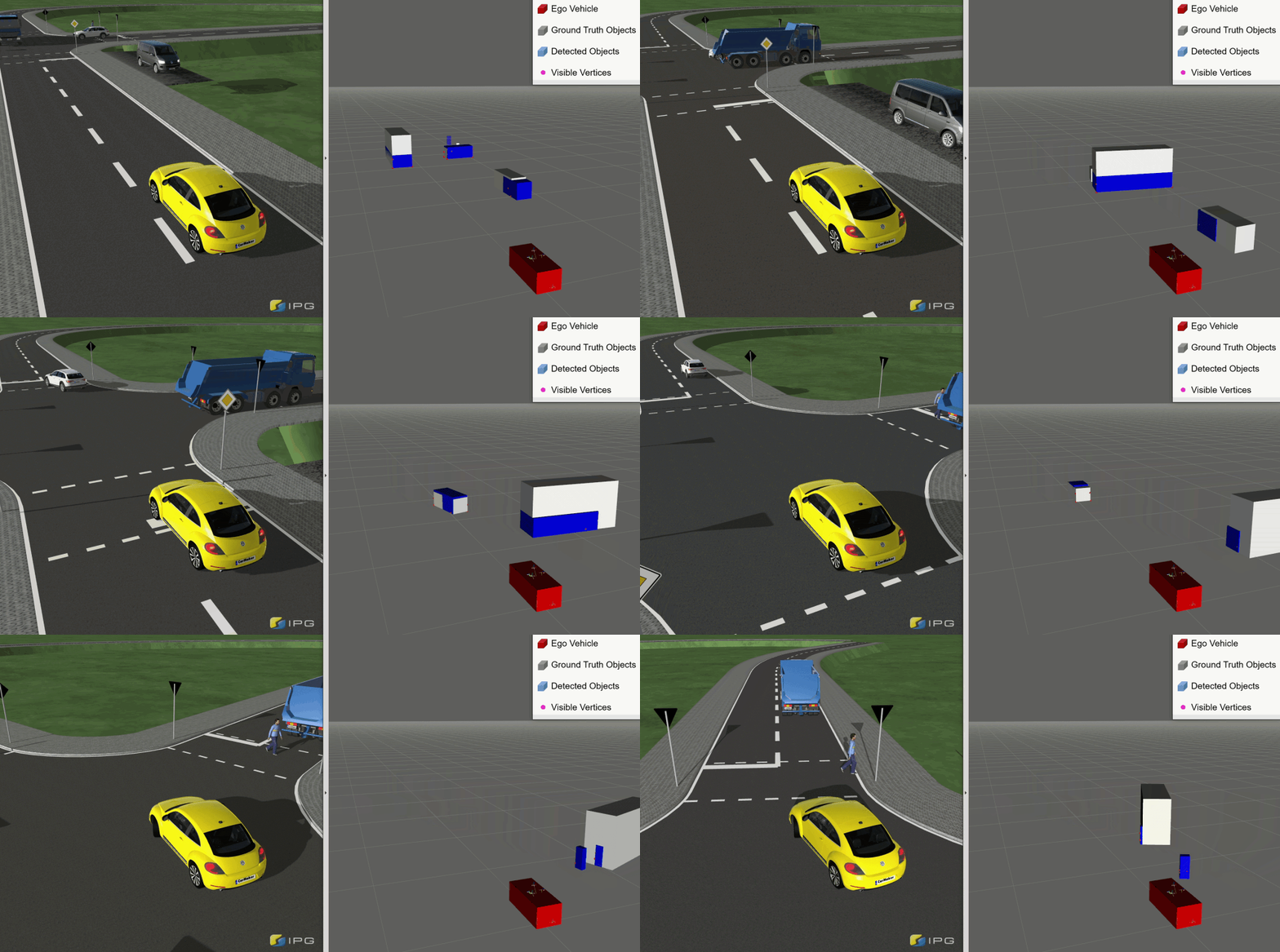
This model is a highly parameterizable generic perception sensor and tracking model. It can be parameterized as a Lidar or a Radar. The model is based on object lists and all modeling is performed on object level. It includes typical sensor artifacts like soft FoV transitions, different detection ranges for different targets, occlusion effects depending on the sensor technology as well as simulation of tracking behavior. The model output are object lists for OSI SenorData moving objects.
The architecture of the model as well as the parameterization structure are designed to be as generic as possible to fit both radar and lidar sensors to utilize similarities in signal propagation and signal processing in both technologies. This way, the model can be parameterized to model different kinds of lidar and radar sensors. To give an example: You can set an irradiation pattern for the modeled sensor. Depending on the sensor technology this can either be an antenna gain pattern for radar or a beam pattern for lidar.
The outer layer of the model is the Modular OSMP Framework by FZD. It specifies ways in which models using the Open Simulation Interface (OSI) are to be packaged for their use in simulation environments using FMI 2.0.
The actual logic of the model is packed in a so-called strategy.
This is where the magic happens.
The apply() function of the strategy is called by the do_calc() function of the Framework.
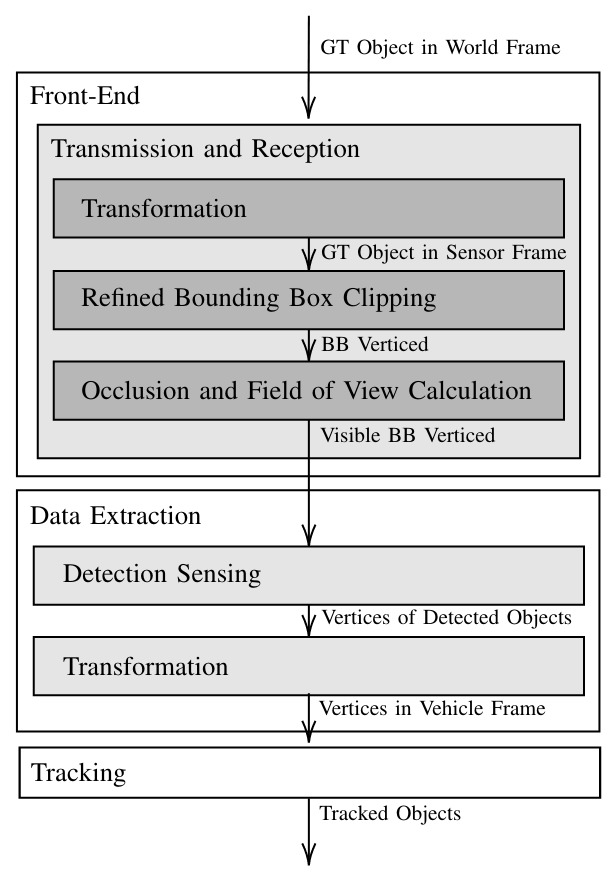
The strategy itself is structured into four modules as shown in the image below.
The first module in the figure above brings the received ground truth stationary and moving objects (potentially also traffic signs and traffic lights from sensor_view.global_ground_truth) into a common format. This enables iterations over all objects regardless of classification. Then they are transformed to the sensor coordinate system for the following calculations.
In the last module, the tracked objects are transformed to the virtual sensor coordinate system (here: vehicle coordinate system) and the fields in the sensor data requested by the HADf are filled.
Requirement analysis revealed mainly three characteristic sensor effects of automotive lidars and radars:
(Partial) occlusion, restricted angular fov, and limited detection range due to the
Then, refined bounding box shapes are generated from the ground truth bounding boxes resulting in a list of characteristic vertices per object.
With these vertices, an occlusion calculation is performed, resulting in the visible 3D vertices of the ground truth objects.
In the detection sensing module, a power equivalent value for every object is calculated.
From the functional decomposition, this would usually be located in the front-end as well,
but as thresholding is directly part of the power calculation, it is situated within the data extraction block.
This calculation is based on externally defined parameters and contains angular fov and range limits by considering irradiation characteristics, visible surfaces, and the
If the power is above a threshold, visible vertices are transformed into the vehicle frame and along with the power calculations passed to the tracking block. There, poses and dimensions from calculated vertices and ground truth are estimated and a tracking logic produces the overall model output.
In the following, a more detailed look at the modules is provided: As mentioned, the first considered effect is object occlusion. To calculate the occlusion, a projection and clipping method is used: Every vertex of the refined bounding boxes of the objects is sorted by distance. Then, for every object all vertices are projected onto a cylinder at unit distance from the sensor and a concave hull is calculated by the concaveman algorithm1, based on2. Consequently, the visible vertices of all objects with their respective outer hull are determined. To calculate the visible area of the polygon for each object, they are sorted by distance and clipped with the Vatti clipping algorithm3. The resulting new vertex points for the hull are reprojected from the 2D cylinder plane onto their original object bounding box to get the desired vertices in 3D space.
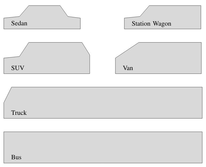
The mentioned refined bounding boxes reflect typical vehicle shapes instead of simple cuboids by considering the shape of the rear and the engine cover. The figure below shows different examples of refined bounding boxes as a side-view. They can be further adapted by adding more vertices to enhance their fidelity, e.g. for the pillar positions, wheels, etc.
The bounding box shapes are selected depending on the ground truth object class and adjusted to the object's dimensions. Consequently, this approach reveals a gap in the OSI definition of vehicle classes. The classification types in OSI refer more to market segments than to the actual vehicle shapes. This should be improved in upcoming releases of the interface standard. Therefore, a separation between sedan and station wagon cannot be accomplished due to the same classification as medium car for vehicles with a length between 4.5 m and 5 m.
To introduce the effect of range - and in case of radar range - measurement noise, the positions of the vertices are altered in range and/or angle by applying parameterizable Gaussian noise.
For lidar simulation, the size of the range-rectified projected area
For radar, instead of the projected area, a typical radar cross-section
$\bar{P}{\text{thres}}=\dfrac{\lambda^2A\text{p,ref}}{r_{\text{max}}^4}$
Detection ranges to standard targets can typically be found in data sheets of commercial radar or lidar sensors.
In most cases, a detection probability for the maximum range is given.
Therefore, Gaussian noise is applied to the threshold with a specified standard deviation , set in the model profile to
This noisy power equivalent threshold simulates the thresholding typically performed in the signal processing of radar and lidar sensors.
If
The vertices are passed to the tracking module as LogicalDetections, so a regular tracking algorithm can be applied on them. Additionally, at a closer look, the vertices reflect the extrema of a lidar point cloud while leaving out the points in between and regular tracking algorithms only select those anyway for object dimension computation. So for tracking, the inner points do not matter and therefore, the object based approach completely suffices in this case. From the vertices at first position, orientation, and dimensions are estimated as the detected object state. The detected objects are compared to a list of previously detected and tracked objects and thereby added, updated or possibly deleted. The track logic can be specified in the model profile. It specifies e.g. the number of consecutive cycles an object has to be detected to create a new track or how many cycles an object is tracked without any detection. Therefore, objects that are hidden now, but where previously detected, are still tracked estimating their movement by either using ground truth information or by predictions based on detected objects of the previous time steps. The estimation of the object dimensions is also considered and filtered over several cycles. If an object is no longer detected over a defined number of cycles, it is deleted from the list. Consideration of the class uncertainties is provided by the model architecture, as well. The output of the tracking module is a list of tracked objects.
The profiles are parameterized in the files profile_*.hpp.in.
The parameters are defined in the files profile.hpp.in.
The profiles can be extended by the strategies with additional parameters and values in their respective folders
as in e.g. src/model/strategies/tracking-strategy/ with profile_struct.hpp.in with the parameters and profile_*.hpp.in with the values.
The profile to be loaded for simulation is set via a model parameter defined in the modelDescription.xml of the FMU.
The first name in src/model/profiles/profile_list.conf is taken as default.
If you would like to have a different one or if your simulation master does not support the configuration of model parameters, you have to adapt the start value of the parameter profile in src/osmp/modelDescription.in.xml.
| Parameter | Description |
|---|---|
| sensor_type | Lidar: 0; Radar: 1 |
| sensor_view_configuration | Update cycle, field of view, physical mounting position w.r.t. center of rear axle, emitter frequency etc. |
| radar_multipath_min_ground_clearance | Minimum ground clearance of an object for a radar to be able to "look underneath" |
| simulate_sensor_failure | if set to 1, sensor will fail after the time set in "stop_detection_time" to simulate sensor failure |
| stop_detection_time | Time in seconds for the sensor to stop detecting objects |
| fov_azimuth_border_stddev | Standard deviation of the normal distribution of the angle (in rad) of the fov. Used for object dimension cropping at the edges |
| fov_elevation_border_stddev | Standard deviation of the normal distribution of the angle (in rad) of the fov. Used for object dimension cropping at the edges |
| vertex_angle_stddev | Standard deviation of the normal distribution of the angle (in rad) of detected vertices of bounding boxes |
| vertex_distance_stddev | Standard deviation of the normal distribution of the distance (in m) of detected vertices of bounding boxes |
| Parameter | Description |
|---|---|
| reference_range_in_m | Detection range for mid-size vehicle (RCS = 10 dBsm) at boreside with a detection probability of 50 % |
| max_range_in_m | Maximum detection range due to physical limits or ambiguity regions |
| irradiation_pattern | Beam pattern for lidar and antenna characteristics for radar as elevation-azimuth-map with normalized values between 0 and 1 |
| detection_thes_dB_stdv | standard deviation for the detection threshold combined with the noise floor |
| Parameter | Description |
|---|---|
| classification_flag | 0 = from ground truth; 1 = all "Unknown Big" |
| orientation_flag | 0 = from ground truth; 1 = from current point cloud segment |
| dimension_and_position_flag | 0 = from ground truth; 1 = from current point cloud segment; 2 = dimension from current point cloud segments with lower bounds, position as center of manipulated pcl segment; 3 = maximum dimension of current and mean of historical point cloud segments, position as center of manipulated pcl segment; 4 = maximum dimension of current and mean of historical point cloud segments with lower bounds, position as center of manipulated pcl segment; |
| minimum_object_dimension | Minimum dimension in m for detected objects |
| historical_limit_dimension | Limits the historical data used for historical mean dimension calculation |
| velocity_flag | 0 = from ground truth; 1 = derivation of position |
| tracking_flag | 0 = ideal (track all ground truth objects); 1 = realistic lidar tracking behavior |
| existence_probability_threshold_for_tracking | Threshold for existence probability, tracking is enabled above threshold |
| min_detections_in_segment_for_tracking | Minimum no. of detections per segment to track it |
| existence_probability_increment | Increment for existence probability |
| existence_probability_decrement | Decrement for existence probability |
The model's name (in this case "ObjectBasedLidarObjectModel") used for CMake-projects and the FMU at the end is defined in file model_name.conf located at src/model.
When building and installing, the framework will build an FMU package into FMU_INSTALL_DIR, which can be used with a simulation tool that supports OSI and fills the required fields listed below.
The parameter variableNamingConvention for the FMU specified within the modelDescription.xml is taken from file variableNamingConvention.conf located at src/osmp.
Possible values are "flat" or "structured".
Required SensorViewConfiguration (parameterized in profile_*.hpp.in) to be Set in the Simulation Tool
- For every simulated physical sensor system:
- sensor_view_configuration.mounting_position.position
- sensor_view_configuration.mounting_position.orientation
- sensor_view_configuration.update_cycle_time
- sensor_view_configuration.range
- sensor_view_configuration.field_of_view_horizontal
- sensor_view_configuration.field_of_view_vertical
- sensor_view.mounting_position
- sensor_view.global_ground_truth.timestamp
- sensor_view.global_ground_truth.host_vehicle_id
- sensor_view.global_ground_truth.stationary_object.id
- sensor_view.global_ground_truth.stationary_object.base.position
- sensor_view.global_ground_truth.stationary_object.base.orientation
- sensor_view.global_ground_truth.stationary_object.base.dimension
- sensor_view.global_ground_truth.stationary_object.classification.type
- sensor_view.global_ground_truth.moving_object.id
- sensor_view.global_ground_truth.moving_object.base.position
- sensor_view.global_ground_truth.moving_object.base.orientation
- sensor_view.global_ground_truth.moving_object.base.orientation_rate
- sensor_view.global_ground_truth.moving_object.base.velocity
- sensor_view.global_ground_truth.moving_object.base.dimension
- sensor_view.global_ground_truth.moving_object.type
- sensor_view.global_ground_truth.moving_object.vehicle_classification.type
- sensor_view.global_ground_truth.moving_object.vehicle_attributes.bbcenter_to_rear
- sensor_view.global_ground_truth.moving_object.vehicle_attributes.ground_clearance
NOTE: Currently, all information on model input is passed to the output.
- sensor_data.timestamp
- sensor_data.moving_object_header.measurement_time
- sensor_data.moving_object_header.cycle_counter
- sensor_data.moving_object_header.data_qualifier
- sensor_data.moving_object.header.ground_truth_id
- sensor_data.moving_object.header.tracking_id
- sensor_data.moving_object.header.age
- sensor_data.moving_object.base.position
- sensor_data.moving_object.base.orientation
- sensor_data.moving_object.base.orientation_rate
- sensor_data.moving_object.base.velocity
- sensor_data.moving_object.base.acceleration
- sensor_data.moving_object.base.dimension
- sensor_data.moving_object.reference_point
- sensor_data.moving_object.movement_state
- sensor_data.moving_object.candidate.probability
- sensor_data.moving_object.candidate.type
- Install cmake
- Install protobuf for MSYS-2020 or Visual Studio 2017
-
Clone this repository with SSH incl. submodules:
git clone git@github.com:openMSL/object_based_generic_perception_object_model.git --recurse-submodules
-
Build the model in MSYS-2020 or Visual Studio 2017
-
Take FMU from
FMU_INSTALL_DIR(Please note that sources are not packed into the FMU at the moment.)
- Install cmake 3.12
- as told in these install instructions
- Install protobuf 3.0.0:
-
Check your version via
protoc --version. It should output:libprotoc 3.0.0 -
If needed, you can install it via
sudo apt-get install libprotobuf-dev protobuf-compiler -
or from source:
- Download protobuf and extract the archive.
- Try to run
./autogen.sh, if it fails, download the gmock-1.7.0.zip, extract it into the protobuf folder and rename the gmock-1.7.0 folder to gmock. - Proceed with the installation with
make
sudo make install
sudo ldconfig # refresh shared library cache.
-
-
Clone this repository with SSH incl. submodules:
git clone git@github.com:openMSL/object_based_generic_perception_object_model.git --recurse-submodules
-
Build the model by executing in the extracted project root directory:
 mkdir cmake-build
 cd cmake-build
 # If FMU_INSTALL_DIR is not set, CMAKE_BINARY_DIR is used
 cmake -DCMAKE_BUILD_TYPE=Release -DFMU_INSTALL_DIR:PATH=/tmp ..
 make -j N_JOBS
-
Take FMU from
FMU_INSTALL_DIR(Please note that sources are not packed into the FMU at the moment.)
C. Linnhoff, P. Rosenberger, and H. Winner, “Refining Object-Based Lidar Sensor Modeling — Challenging Ray Tracing as the Magic Bullet,” IEEE Sensors Journal, Volume 21, Issue 21, Nov. 1, 2021
If you find our work useful in your research, please consider citing:
@ARTICLE{linnhoff2021,
  author={Linnhoff, Clemens and Rosenberger, Philipp and Winner, Hermann},
  journal={IEEE Sensors Journal},
  title={Refining Object-Based Lidar Sensor Modeling — Challenging Ray Tracing as the Magic Bullet},
  year={2021},
  volume={21},
  number={21},
  pages={24238-24245},
  doi={10.1109/JSEN.2021.3115589}
}
This work received funding from the research project "SET Level" of the PEGASUS project family, promoted by the German Federal Ministry for Economic Affairs and Energy based on a decision of the German Bundestag.
| SET Level | PEGASUS Family | BMWi |
|---|---|---|
We would like to thank Yifei Jiao for his contribution to the first prototype.
Thanks also to all contributors of the following libraries:
- Open Simulation Interface, a generic interface based on protocol buffers for the environmental perception of automated driving functions in virtual scenarios
- FMI Version 2.0: FMI for Model Exchange and Co-Simulation
- Eigen, a C++ template library for linear algebra: matrices, vectors, numerical solvers, and related algorithms.
- Concaveman, an algorithm for concave hull generation
- Clipper, an open-source polygon clipping algorithm (Boost Software License V1.0)
1: V. Agafonkin. (2016) Conacveman. [Online]. Available: https://github.com/mapbox/concaveman
2: J.-S. Park and S.-J. Oh, “A new concave hull algorithm and concaveness measure for n-dimensional datasets,” Journal of Information Science and Engineering, vol. 29, no. 2, p. 19, 2013.
3: B. R. Vatti, “A generic solution to polygon clipping,” Communications of the ACM, vol. 35, no. 7, pp. 56–63, 1992.


