Julia for Numerical Computation in MIT Courses

Several MIT courses involving numerical computation, including 18.06, 18.303, 18.330, 18.335/6.337, 18.337/6.338, and 18.338, are beginning to use Julia, a fairly new language for technical computing. This page is intended to supplement the Julia documentation with some simple tutorials on installing and using Julia targeted at MIT students. See also our Julia cheatsheet listing a few basic commands, as well as the Learn Julia in Y minutes tutorial page.

In particular, we will be using Julia in the IJulia browser-based enviroment, which leverages your web browser and IPython to provide a rich environment combining code, graphics, formatted text, and even equations, with sophisticated plots via Matplotlib.

See also Viral Shah's Julia slides and the January 2013 Julia Tutorial videos.

Why Julia?

Traditionally, these sorts of courses at MIT have used Matlab, a high-level environment for numerical computation. Other possibilities might be Scientific Python (the Python language plus numerical libraries), GNU R, and many others. Julia is another high-level free/open-source language for numerical computing in the same spirit, with a rich set of built-in types and libraries for working with linear algebra and other types of computations, with a syntax that is superficially reminiscent of Matlab's.

High-level dynamic programming languages (as opposed to low-level languages like C or static languages like Java) are essential for interactive exploration of computational science. They allow you to play with matrices, computations on large datasets, plots, and so on without having to worry about managing memory, declaring types, or other minutiae—you can open up a window and start typing commands to immediately get results.

The traditional problem with high-level dynamic languages, however, is that they are slow: as soon as you run into a problem that cannot easily be expressed in terms of built-in library functions operating on large blocks of data ("vectorized" code), you find that your code is suddenly orders of magnitude slower that equivalent code in a low-level language. The typical solution has been to switch to another language (e.g. C or Fortran) to write key computational kernels, calling these from the high-level language (e.g. Matlab or Python) as needed, but this is vastly more difficult than writing code purely in a high-level language and imposes a steep barrier on anyone hoping to transition from casual experimentation to "serious" numerical computation. Julia mostly eliminates this issue, because it is carefully designed to exploit a "just-in-time compiler" called LLVM, making it possible to write high-level code in Julia that achieves near-C speed. (It also means that we can perform meaningful performance experiments easily in courses where this matters, e.g. in 18.335.)

Speed, while avoiding the "two-language" problem of requiring C or Fortran for critical code, is the initial draw of Julia, but there are a few other nice points. Unlike Matlab, it is free/open-source software, which eliminates licensing headaches and allows you to look inside the Julia implementation to see how it works (since Julia is mostly written in Julia, its code is much more readable than a language like Python that is largely implemented in low-level C). For calling existing code, it has easy facilities to call external C or Fortran libraries or to call Python libraries. Multiple dispatch makes it especially easy to overload operations and functions for new types (e.g. to add new vector or numeric types). Julia's built-in metaprogramming facilities make it easy to write code that generates other code, essentially allowing you to extend the language as needed. And so on...

Using Julia on juliabox

The simplest way to use Julia is to go to juliabox.com. Once you log in (e.g. with a gmail account), you can run Julia code online (on Amazon Cloud servers) via the browser-based Jupyter notebook interface without installing anything on your computer.

Although you wouldn't want to run large computations on juliabox, it should be fine for simple homework problems.

Installing Julia and IJulia

If you use Julia enough, you'll eventually want to install it on your own computer. Your code will run faster and won't require a network connection, but can still use the same browser-based notebook interface.

First, download the current release of Julia version 0.6.x and run the installer. Then run the Julia application (double-click on it); a window with a julia> prompt will appear. At the prompt, type:

Pkg.add("IJulia")

You may also want to install these packages, which we tend to use in a lot of the lecture materials:

Pkg.add("Interact")
Pkg.add("PyPlot")

Then you can launch the notebook by running

using IJulia
notebook()

at the julia> prompt, as described below.

(An alternative is to download the JuliaPro package, which includes Julia, IJulia, the Juno IDE based on the Atom editor, and a number of packages pre-installed.)

Troubleshooting:

If you ran into a problem with the above steps, after fixing the problem you can type Pkg.build() to try to rerun the install scripts.
If you tried it a while ago, try running Pkg.update() and try again: this will fetch the latest versions of the Julia packages in case the problem you saw was fixed. Run Pkg.build("IJulia") if your Julia version may have changed. If this doesn't work, try just deleting the whole .julia directory in your home directory (on Windows, it is called AppData\Roaming\julia\packages in your home directory) and re-adding the packages.
On MacOS, you currently need MacOS 10.7 or later; MacOS 10.6 doesn't work (unless you compile Julia yourself, from source code).
Internet Explorer 8 (the default in Windows 7) or 9 don't work with the notebook; use Firefox (6 or later) or Chrome (13 or later). Internet Explorer 10 in Windows 8 works (albeit with a few rendering glitches), but Chrome or Firefox is better.
If the notebook opens up, but doesn't respond (the input label is In[*] indefinitely), try creating a new Python notebook (not Julia) from the New button in the Jupyter dashboard, to see if 1+1 works in Python. If it is the same problem, then probably you have a firewall running on your machine (this is common on Windows) and you need to disable the firewall or at least to allow the IP address 127.0.0.1. (For the Sophos endpoint security software, go to "Configure Anti-Virus and HIPS", select "Authorization" and then "Websites", and add 127.0.0.1 to "Authorized websites"; finally, restart your computer.)

Julia on MIT Athena

Julia is also installed on MIT's Athena Computing Environment. Any MIT student can use the computers in the Athena Clusters on campus, and you can also log in remotely to athena.dialup.mit.edu via ssh. (Note: the linux.mit.edu dialup does not work with Julia.)

In the terminal of an Athena machine, type:

add julia

to load the Julia and IPython software locker.

The first time you use Julia on Athena, you will need to set up IJulia: run julia, and at the julia> prompt, type

Pkg.update()
Pkg.add("PyPlot")
Pkg.add("IJulia")

Thereafter, you can run the notebook as below.

(Unfortunately, as of this writing Athena still has IPython version 2, whereas IJulia requires IPython version 3 or later, so you can't use the ipython on Athena.)

Remote access to Julia on Athena.

If you are logging in remotely to athena.dialup.mit.edu, you can use a trick called "port forwarding" to run IJulia in your local web browser (MUCH faster and nicer than running a web browser remotely over X Windows). The steps are:

Log in by typing ssh -L 8778:localhost:8998 athena.dialup.mit.edu into your terminal. (This works with Macs and GNU/Linux; how you do it on Windows will depend upon your ssh client and whether it supports port forwarding: you want to forward port 8998 on the remote machine to port 8778 on localhost.)
add julia and make sure IJulia is installed as above.
Quit Julia and type (at the Athena prompt): ipython notebook --no-browser ... unfortunately, this won't work until Athena installs a newer version of ipython. Instead of ipython, you can find the jupyter notebook command that Julia installs by running using IJulia; join(IJulia.notebook_cmd, " ") in Julia.
In your ordinary web browser, type localhost:8778 in the address bar.

You should see the IPython dashboard for IJulia running on Athena (creating a new notebook will create the file in your Athena account).

Updating Julia and IJulia

Julia is improving rapidly, so it won't be long before you want to update to a more recent version. The same is true of Julia add-on packages like PyPlot. To update the packages only, keeping Julia itself the same, just run:

Pkg.update()

at the Julia prompt (or in IJulia).

If you download and install a new version of Julia from the Julia web site, you will also probably want to update the packages with Pkg.update() (in case newer versions of the packages are required for the most recent Julia). In any case, if you install a new Julia binary (or do anything that changes the location of Julia on your computer), you must update the IJulia installation (to tell IPython where to find the new Julia) by running Pkg.build("IJulia") at the Julia command line (not in IJulia).

Running Julia in the IJulia Notebook

Once you have followed the installation steps above, open up the Julia command line (run julia or double-click the julia program) and run

using IJulia
notebook()

(You will have to leave the Julia command-line window open in order to keep the IJulia/Jupyter process running. Alternatively, you can run notebook(detached=true) if you want to run the Jupyter server as a background process, at which point you can close the Julia command line, but then if you ever want to restart the Jupyter server you will need to kill it manually.

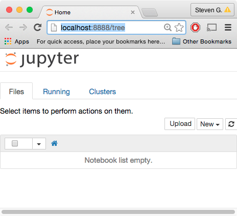
A "dashboard" window like this should open in your web browser (at address localhost:8888, which you can return to at any time as long as the notebook() server is running; I usually keep it running all the time):

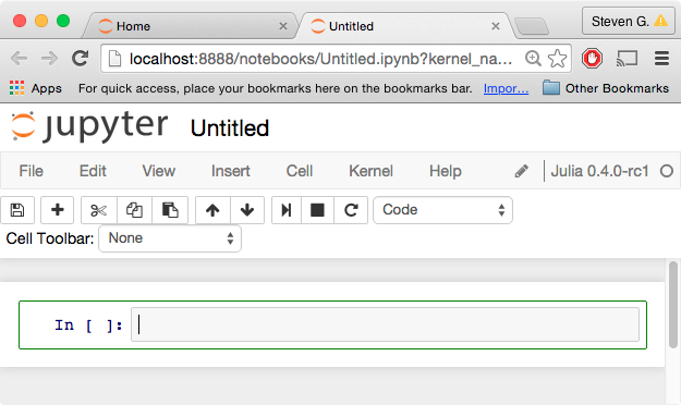
Now, click on the New button and select the Julia option to start a new "notebook". A notebook will combine code, computed results, formatted text, and images; for example, you might use one notebook for each problem set. The notebook window that opens will look something like:

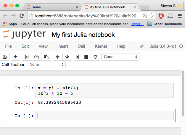
You can click the "Untitled" at the top to change the name, e.g. to "My first Julia notebook". You can enter Julia code at the In[ ] prompt, and hit shift-return to execute it and see the results. If you hit return without the shift key, it will add additional lines to a single input cell. For example, we can define a variable x (using the built-in constant pi and the built-in function sin), and then evaluate a polynomial 3x^2 + 2x - 5 in terms of x (note that, unlike Matlab or Python, we don't have to type 3*x^2 if we don't want to: a number followed by a variable is automatically interpreted as multiplication without having to type *):

The result that is printed (in Out[1]) is the last expression from the input cell, i.e. the polynomial. If you want to see the value of x, for example, you could simply type x at the second In[ ] prompt and hit shift-return.

See, for example, the mathematical operations in the Julia manual for many more basic math functions.

Plotting

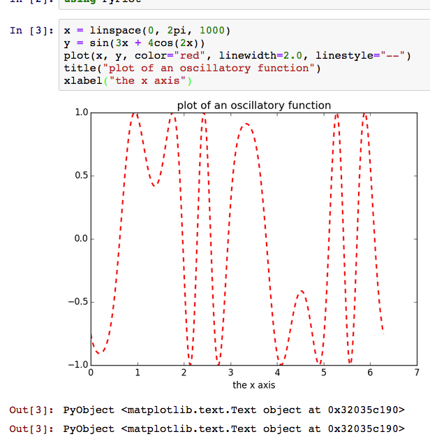
There are several plotting packages available for Julia. If you followed the installation instructions, above, you already have one full-featured Matlab-like plotting package installed: PyPlot, which is simply a wrapper around Python's amazing Matplotlib library.

To start using PyPlot to make plots in Julia, first type using PyPlot at an input prompt and hit shift-enter. using is the Julia command to load an external module (which must usually be installed first, e.g. by the Pkg.add("PyPlot") command from the installation instructions above). The very first time you do this, it will take some time; in Julia 0.4 or later, the module and its dependencies will be "precompiled" so that in subsequent Julia sessions it will load quickly.

Then, you can type any of the commands from Matplotlib, which includes equivalents for most of the Matlab plotting functions. For example:

Printing/exporting Notebooks

Currently, printing a notebook from the browser's Print command can be somewhat problematic. There are four solutions:

At the top of the notebook, click on the File menu (in the notebook, not the browser's global menu bar), and choose Print Preview. This should open up a window/tab that you can print normally.
For turning in homework, a class may allow you to submit the notebook file (.ipynb file) electronically (the graders will handle printing). You can save a notebook file in a different location by choosing Download as from the notebook's File menu.
The highest-quality printed output is produced by IPython's nbconvert utility. For example, if you have a file mynotebook.ipynb, you can run ipython nbconvert mynotebook.ipynb to convert it to an HTML file that you can open and print in your web browser. This requires you to install IPython, Sphinx (which is automatically installed with the Anaconda Python/IPython distribution), and Pandoc on your computer.
If you post your notebook in a Dropbox account or in some other web-accessible location, you can paste the URL into the online nbviewer to get a printable version.

pkraison/julia-mit