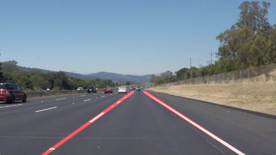
This project is developed to identify the lane lines on the road. A pipeline is created to test the result initially on images and later applied the results to video stream(series of images).
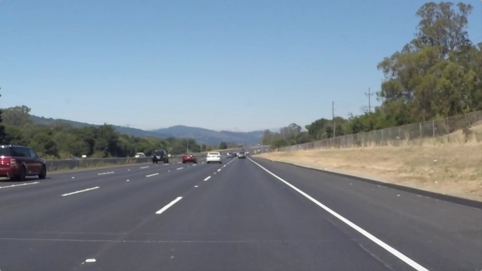
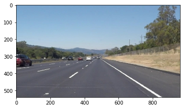
Raw image of a road.
Identified lane line of the road.
The pipeline for image consist of 6 steps-
It reads the image of road whose lane line we have to find.
#reading in an image
image = mpimg.imread('test_images/solidWhiteRight.jpg')

#printing out some stats and plotting
print('This image is:', type(image), 'with dimensions:', image.shape)
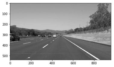
plt.imshow(image) # if you wanted to show a single color channel image called 'gray', for example, call as plt.imshow(gray, cmap='gray')grayscale() function is used to convert the test_image to the grayscaled image. This function uses the cv2.cvtColor() opencv function which convert images from one color space to another.
#show the grayscaled image
gray = grayscale(image)
plt.imshow(gray, cmap='gray')Here we have also included gaussian_blur function which is used for the Gaussina smooting, a way of suppressing noise and spurious gradient.
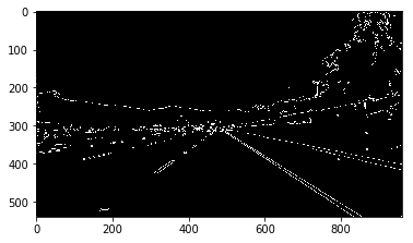
Then canny() function is used to convert gray image to edges image. Here it uses the cv2.canny() opencv function which returns a binary image with white pixels tracing out the detected edges and black everywhere else.
# apply Gaussian smoothing
blur_gray = gaussian_blur(gray, 3)

#show the edges image
edges = canny(blur_gray, 50, 150)
plt.imshow(edges, cmap='gray')The region_of_interest() function is used to mask a area according to your desired shape in a image. Here we have used a quardilateral shaped masking region with following vertices.
#show masked edges
vertices = np.array([[(150, 540),(450, 315), (500, 315), (880, 540)]])
masked_edges = region_of_interest(edges, vertices)
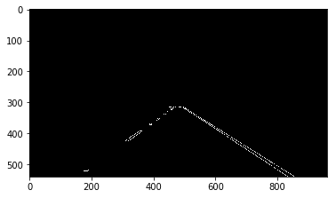
plt.imshow(masked_edges, cmap='gray')rho = 1 # distance resolution in pixels of the Hough grid
theta = np.pi/180 # angular resolution in radians of the Hough grid
threshold = 15 # minimum number of votes (intersections in Hough grid cell)
min_line_len = 40 #minimum number of pixels making up a line
max_line_gap = 20 # maximum gap in pixels between connectable line segments
# Run Hough on edge detected image
line_img = hough_lines(masked_edges, rho, theta, threshold, min_line_len, max_line_gap)
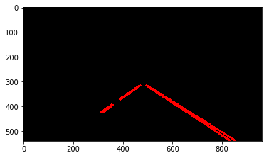
plt.imshow(line_img)Before changing in draw_line() function the output of hough_lines() was like -
But in order to draw a single line for the left and right lane the `draw_line()` function has been modified to -
def draw_lines(img, lines, color=[255, 0, 0], thickness=2):

    left_line_slopes = []
    right_line_slopes = []
    left_line_pts = []
    right_line_pts = []

    left_x_pts = []
    left_y_pts = []
    right_x_pts = []
    right_y_pts = []

#     Store the slope of each line in an array.
    for line in lines:
        for x1,y1,x2,y2 in line:
            if((y2-y1)/(x2-x1) < 0):
                left_line_slopes.append(round(((y2-y1)/(x2-x1))*10))
            else:
                right_line_slopes.append(round(((y2-y1)/(x2-x1))*10))

#     Initializes variables to empty string.
    most_left_pt_freq = ''
    most_right_pt_freq = ''

#     Find which slope has the maximum frequency.
    if len(left_line_slopes):
        most_left_pt_freq = max(set(left_line_slopes), key=left_line_slopes.count)

    if len(right_line_slopes):
        most_right_pt_freq = max(set(right_line_slopes), key=right_line_slopes.count)

#     Check that if slope of line is in range, then save its point in an array
    for line in lines:
        for x1,y1,x2,y2 in line:
            if not most_left_pt_freq is '':
                if((most_left_pt_freq-1) <= (round(((y2-y1)/(x2-x1))*10)) <= (most_left_pt_freq+1)):
                    left_line_pts.append((x1,y1))
                    left_line_pts.append((x2,y2))
    if not most_left_pt_freq is '':
        for x1,y1 in left_line_pts:
            left_x_pts.append(x1)
            left_y_pts.append(y1)

#         Calculating y coordinates of the end points of left line
        left_y1 = min(left_y_pts)
        left_y2 = img.shape[0]

#         Calculate m and b for the left lines(y=mx+b)
        left_m, left_b = np.polyfit(left_x_pts, left_y_pts, 1)

#         Calculate x coordinates of the end points of left line.
        left_x1 = int((left_y1 - left_b)/left_m)
        left_x2 = int((left_y2 - left_b)/left_m)

#         Draw left lines
        cv2.line(img, (left_x1, left_y1), (left_x2, left_y2), (255, 0, 0), 5)

#     Check that if slope of line is in range, then save its point in an array
    for line in lines:
        for x1,y1,x2,y2 in line:
            if not most_right_pt_freq is '':
                if((most_right_pt_freq-1) <= (round(((y2-y1)/(x2-x1))*10)) <= (most_right_pt_freq+1)):
                    right_line_pts.append((x1,y1))
                    right_line_pts.append((x2,y2))

    if not most_right_pt_freq is '':
        for x1,y1 in right_line_pts:
            right_x_pts.append(x1)
            right_y_pts.append(y1)

#         Calculating y coordinates of the end points of right line.
        right_y1 = min(right_y_pts)
        right_y2 = img.shape[0]

#         Calculate m and b for the lines(y=mx+b)
        right_m, right_b = np.polyfit(right_x_pts, right_y_pts, 1)

#         Calculate x coordinates of the end points of right line.
        right_x1 = int((right_y1 - right_b)/right_m)
        right_x2 = int((right_y2 - right_b)/right_m)

#         Draw right lines
        cv2.line(img, (right_x1, right_y1), (right_x2, right_y2), (255, 0, 0), 5)
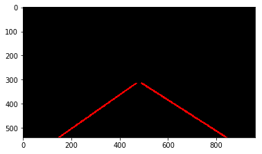
After modifying draw_line() the output of hough_lines() gets` updated to -
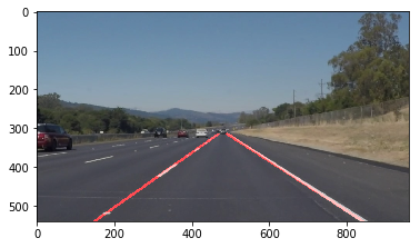
Weighted_img() uses the cv2.addWeighted() opencv function which returns the added weighted sum of the array of two images i.e line image and raw image.
#show lines
line_edges = weighted_img(line_img, image, 0.8, 1, 0)
plt.imshow(line_edges)
mpimg.imsave('test_images/whiteCarLaneSwitch_final.jpg', line_edges)The pipeline for video contain one step-
def process_image(image):

    #show the grayscaled image
    gray = grayscale(image)

    #show the edges image
    blur_gray = gaussian_blur(gray, 3)
    edges = canny(blur_gray, 50, 150)

    #show masked edges
    vertices = np.array([[(150, 540),(450, 315), (500, 315), (880, 540)]])
    masked_edges = region_of_interest(edges, vertices)

    #show hugh lines
    rho = 1 # distance resolution in pixels of the Hough grid
    theta =  np.pi/180 # angular resolution in radians of the Hough grid
    threshold = 1     # minimum number of votes (intersections in Hough grid cell)
    min_line_len = 40 #minimum number of pixels making up a line
    max_line_gap = 20    # maximum gap in pixels between connectable line segments

    line_img = hough_lines(masked_edges, rho, theta, threshold, min_line_len, max_line_gap)

    #show lines
    line_edges = weighted_img(line_img, image, 0.8, 1, 0)

    return line_edges