Binarena ("bin arena") is an interative visualizer of metagenomic assembly that facilitates observation, semi-manual and semi-automatic binning of metagenomic contigs.
Please check out this live demo. It is a fully functional program with a pre-loaded sample dataset. You may close the data, then drag and drop your own data into the interface and start to analyze!
- Installation | main interface | system requirements | mouse and keyboard shortcuts
- Input files: data table | table view | special columns | additional data
- Display items: legends and data scaling | data transformation | color coding | image export
- Contig selection | masking | highlighting | summary | search | mini plot
- Binning plan | table of bins | from selection to bin
- Binning confidence evaluation | binning plan comparison
- FAQ | contact
Download this program, unzip, and double-click "BinaRena.html". That's it!
BinaRena is a client-end web application. It is written in vanilla JavaScript, with minimum usage of third-party libraries, which are all bundled in the package. it does not require installation, nor does it require a web server running in the backend. In other words, it is literally a webpage running in your browser.
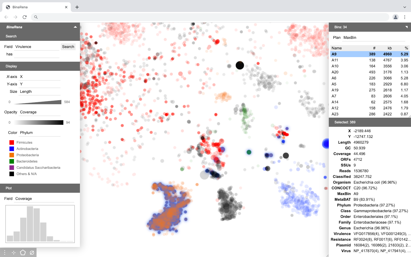
The main interface of BinaRena is an interactive scatter plot. It focuses on the display while minimizing other visual elements to let the user concentrate on the research task. Panels can be expanded / hidden on demand. Most functions (buttons) are only visible when the user moves the mouse over relevant items.
Here is the fully expanded main interface of BinaRena.
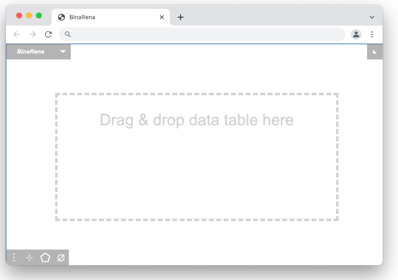
Here is the default interface when the program starts.
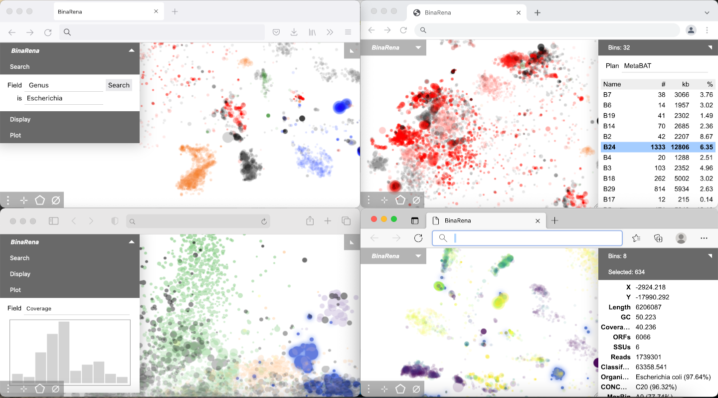
BinaRena runs in most modern web browsers, including Chrome, Firefox, Edge, and Safari (see screenshots below). A typical laptop is sufficient for running BinaRena.
The BinaRena interface is like a digital map and is very intuitive. While although operations can be triggered through the graphical interface, the following basic operations are most convenient by using your mouse and keyboard.
- Drag the plot or use arrow keys (
←,↑,→and↓) to move around. - Zoom in/out: Mouse wheel, or use
=and-. - Click a contig to select it. Hold
Shiftand click to select multiple contigs. - Click a selected contig to unselect it. Hold
Shiftand click to unselect multiple contigs. - Press
Enterto enter polygon selection mode. Then use mouse clicks to draw a polygon to contain multiple contigs. PressEnteragain to complete selection. HoldShiftwhile pressing the secondEnterto add contigs to the existing selection. - Press
DeleteorBackspaceto mask selected contigs. PressZto undo. - Presee
Lto highlight selected contigs. - Press
Spaceto create a new bin from selected contigs. - Click a bin name to select it and all member contigs. Click it again to edit its name. Hold Shift and click to select multiple bins.
- Press
.(>) to add selected contigs to the current bin, press,(<) to remove selected contigs from the current bin, press/to update the current bin with selected contigs (i.e., replace its content). - Press
0to reset the plot view.
BinaRena operates on one dataset at a time. A dataset is an entire metagenomic assembly, i.e., a collection of contigs (this document does not differentiate contigs and scaffolds). The information being handled is the properties of individual contigs.
To load a dataset, simply drag and drop the file into the blank program window.
The most typical input file format is a data table (tab-delimited file, or TSV) that stores properties of contigs (scaffolds) in an assembly. Here is an example.
Each row represents one contig. The first column must be unique contig identifiers. The remaining columns are arbitrary properties (such as length, coverage, GC%, taxonomy, etc.). These fields may be in any of the following four types:
- number(
n), category(c), feature(f), description(d)
The program will guess column type based on the data. To be safer, you may append a type code to a column name following a pipe (|), such as "genes|n" and "plasmid|c".
In a feature-type column, a cell can have multiple comma-separated features, such as "Firmicutes,Proteobacteria,Cyanobacteria".
One may assign a weight to each category or feature, using a numeric suffix following a colon (:), such as "Ruminococcus:80", and "rpoB:1,dnaK:2,16S:5".
This weight can represent quantity, proportion, confidence, etc.
Empty cells will be treated as missing values.
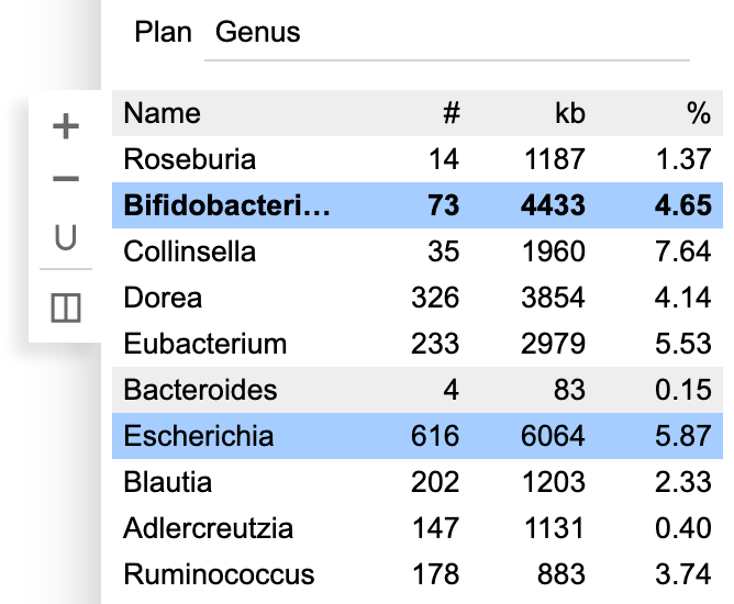
One can click Show data from the context menu to open a window to browse the current dataset. Alternatively, when one or more bins are selected, one can click the ◫ button in the bin table toolbar to browse the data of contigs within these bins. Click Export to save the data table as a TSV file.
When a data table is loaded, BinaRena attempts to "guess" the meaning of data columns by their name and type, and displays the most relevant information. Specifically, the following fields and keyword patterns are recognized:
- Length (bp): "length", "size", "len", "bp", etc.
- Coverage (x): "coverage", "depth", "cov", etc.
- GC content (%): "gc", "g+c", "gc%", "gc-content", etc.
- X- (and y-axes) (if available): "x", "xaxis", "x1", "axis1", "dim1", "pc1", "tsne1", "umap1", etc.
The matching process is case-insensitive. Suffixes after common delimiters (" ", "/", "_", ".") are stripped. For examples, Length (bp) and size_of_scaffold will be recognized as length.
It isn't a problem if the program misses a special column (which is very possible). One can always manually choose the most relevant display items.
When a dataset has been opened, one may append additional data files to it simply by dragging and dropping them into the interface. They will be filter to match the current contig IDs (first column) and appended to the right of the current data table.
BinaRena supports several special file types that are frequently generated in typical metagenomic data analysis workflows.
An assembly file is a FASTA format file containing multiple contig sequences. BinaRena can read DNA sequences and calculate length and GC content of each contig. If this file is generated by SPAdes or MEGAHIT, BinaRena can recognize coverage from sequence titles.
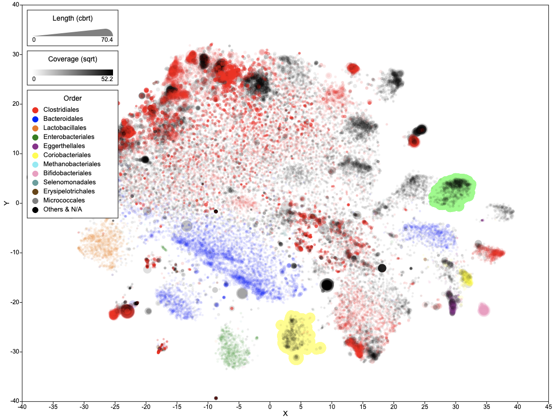
BinaRena is an interactive scatter plot of contigs, with five display items:
- x-axis, y-axis, size (radius of contig), opacity (alpha value), and color.
Each display item can be changed and tweaked in the display panel. When the user moves the mouse of an item, two button will emerge, one letting the user select a data transformation method, and the other letting the user display a legend.
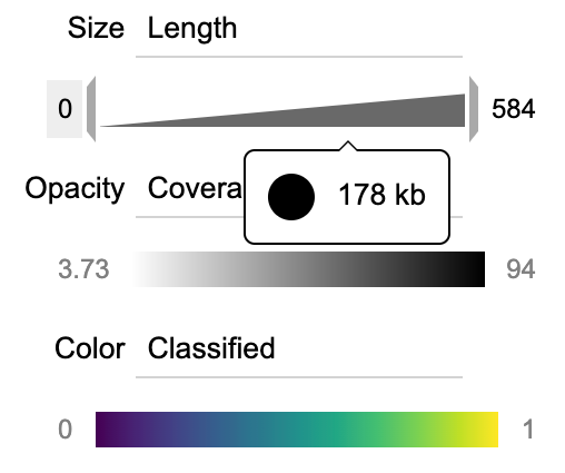
BinaRena provides interactive legends to inform the user of the (numeric) data. Move the mouse over the legend to see the original value in real time. Menwhile, two brackets will show up at the edges of the legend. Drag them to modify the displayed range of data. The lower limit is clickable. It lets the user toggle between zero or minimum value in the data.
Biological data are usually highly skewed. To effectively display them, proper transformation is usually necessary. BinaRena provides various transformation methods that can be easily selected from a dropdown menu next to the field selection box.
Specifically, BinaRena supports the following transformations:
- Square, cube, 4th power.
- Square root, cube root, 4th root.
- Logarithm and exponential.
- Logit and arcsine (for proportion data).
- Ranking.
Note: Certain values may become invalid after certain transformation. For example, zero and negative numbers cannot be log-transformed. In such cases, the contigs will be displayed using the default setting (e.g., color is grey).
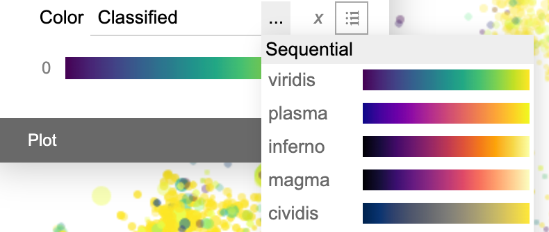
The color panel has an additional dropdown menu to let the user choose from multiple standard color palettes.
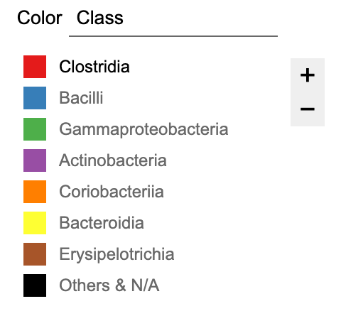
For categorical data, BinaRena automatically identifies and colors the most frequent categories in the dataset, while leaving all remaining categories in black. One may use the floating + and − buttons to increase / decrease the number of colored categories.
The plot rendered by BinaRena can be exported as an image file. There are two options for doing this:
-
Press
Por click the⊹button to take a screenshot of the current view and save as a PNG (portable network graphics) file. -
Mouse over the
⊹button and select "SVG" in the expanded menu. This will generate an SVG (scalable vector graphics) file. It is a vector image therefore it can be further edited in vector image editing programs, such as Inkscape. Compared with PNG which is a bare screenshot, the SVG image has x- and y-axes ticked, labeled, and aligned to "nice" tick numbers, and legends (size, opacity and/or color) displayed in the plot. It is suitable for further processing to generate publication-quality figures.
In the interactive scatter plot, one can simple click circles (contigs) to select them. Hold Shift and click to select multiple. Click selected ones to unselect them.
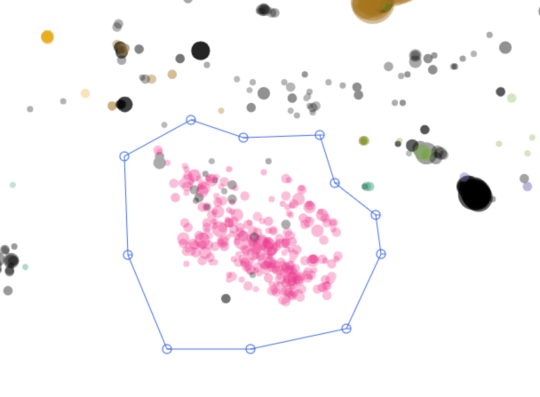
A more efficient may is to press Enter or click the ⬠ button in the corner to enter the polygon selection mode.
Then one can click on the plot to draw a polygon to contain contigs of interest. When done, press Enter again and these contigs will be selected.
Hold Shift when finishing selection will add the contigs to the current selection.
One can press the Delete key or click the ∅ button in the corner to mask currently selected contigs. These contigs will disappear from the plot. They will also be excluded from subsequent operations (e.g., they cannot be selected, nor can they influence calculation of metrics). This function is useful for cloaking unwanted contigs during binning.
The masked contigs are not deleted from the dataset. They can be released back to the view by clicking the × button.
One can also press Z or click the ↩ button to undo previous masking operations one by one. The program allows a total of 50 regrets.
- Note that masked contigs will not be immediated deleted from bins. One can click the ∅ button in the bin table toolbar to remove masked contigs from all bins.
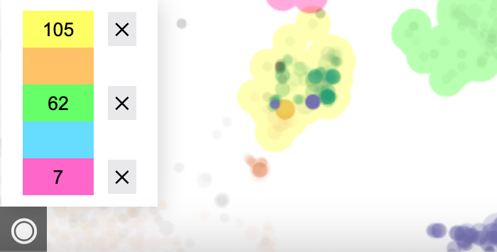
One can press the L key or click the ◉ button in the corner to highlight currently selected contigs. Moreover, one may select one of multiple highlight colors from the menu.
The highlight will stay with the contigs no matter how the layout and display items change, until the user click the × button next to each color to release them.
Highlighting will not affect binning, search, calculation and operations. It serves as a visual annotation of contigs to make them noticeable to the user.
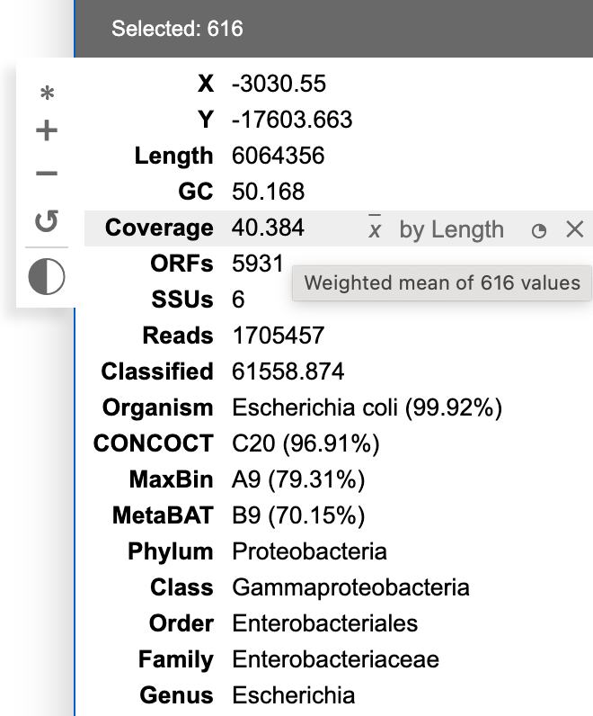
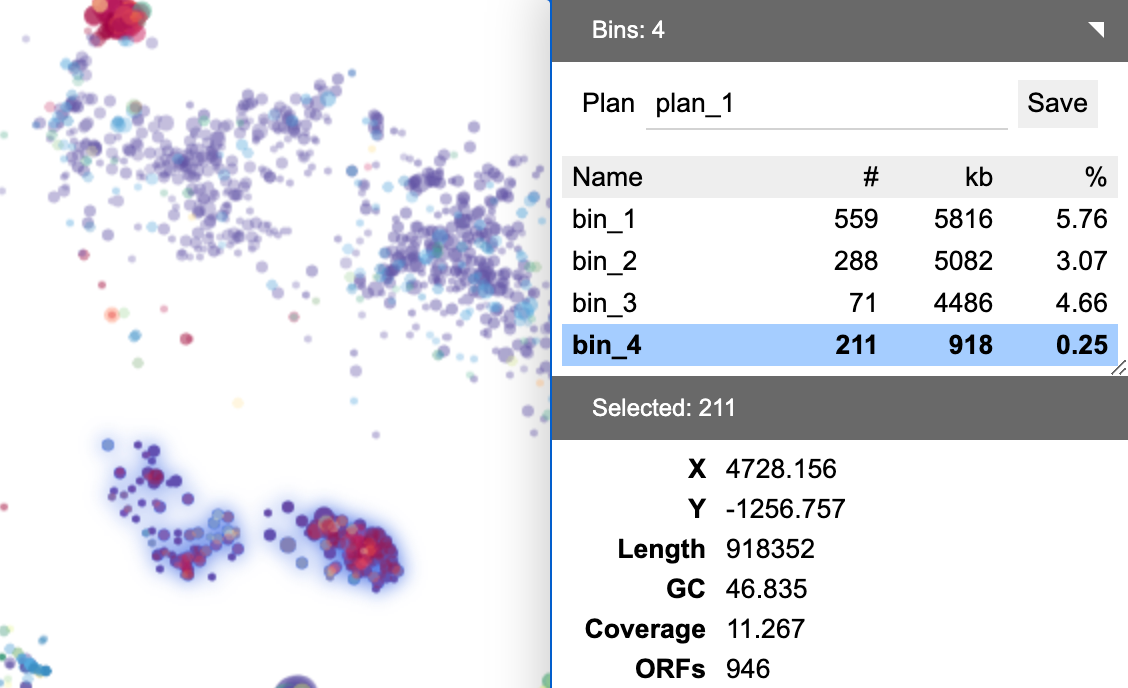
BinaRena displays a summary of properties of the select contigs in real time to let the user see what's included. Each row represents a field. When the user moves the mouse over a row, a mini control panel will show up.
When multiple contigs are selected, the displayed value of numeric fields is calculated using either mean (x) or sum (Σx) of the contigs, optionally weighted by another variable. BinaRena attempts to "guess" the most relevant metric for each column. For examples, "length" should be the sum of lengths of all contigs, whereas "coverage" should be the average of coverages of the contigs, weighted by contig length. One can mouse hover the displayed value to see how it is exactly calculated, and tweak the metrics (in case BinaRena didn't guess right).
For categorical columns, the displayed category is the majority-rule category, if there are multiple options (i.e., the selected contigs are a mixture), determined by weighting against the contig length (one can tweak this). The relative frequency of the main category is displayed in the parentheses. If no category is over half, the row will be displayed as "ambiguous", while the most frequent category can be found in the tooltip during mouse hovering.
One may click the ◔ button in each row to display a histogram of the distribution of this variable in a mini plot.
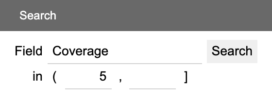
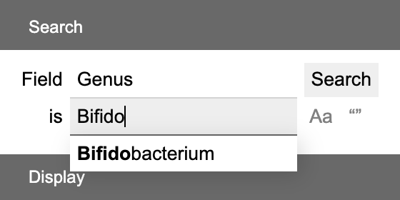
The Search panel offers functions to search the assembly for contigs that match given criteria.
For numeric fields, enter (or leave empty) maximum and minimum thresholds. Click the boundaries to toggle between inclusion (()) and exclusion ([]).
For categorical, feature set and descriptive fields, enter a keyword to search. The keyword box can auto-complete based on current categories and features. Click Aa to toggle case sensitivity and "" to toggle whole/partial matching.
For feature set field, the whole contig will match as long as any feature on it matches.
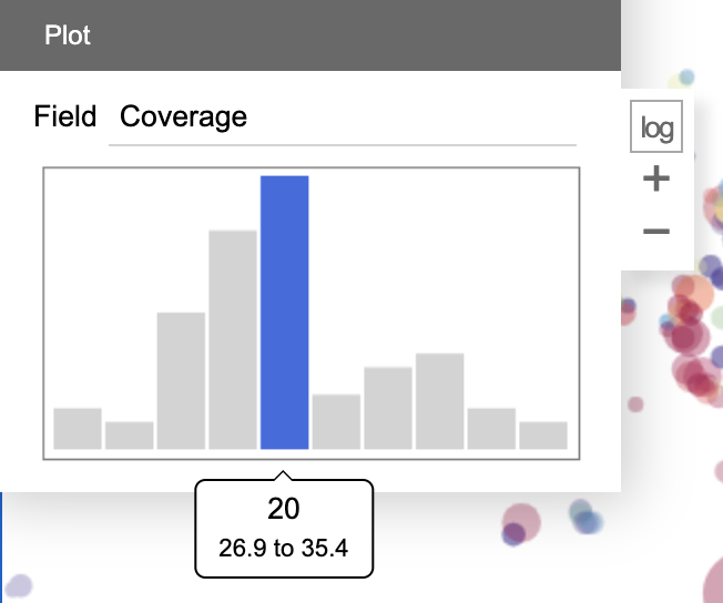
The mini plot panel displays an interactive histogram of a user-chosen variable of the selected contigs. Mouse over the bars to display the range and size of them. Click log to apply log-transformation. Click + and - to increase / decrease the number of bars.
One may use mouse dragging to select a range of bars. The contigs will be filtered down to the selected range.
This miniplot faciliates the user to observe the distribution of the variable in a set of contigs, and further perform filtering based on the observation. For examples, one may remove contaminations from a bin which appear to be outliers in the histogram; one may also separate two closely related strains which show a bimodal distribution in the histogram.
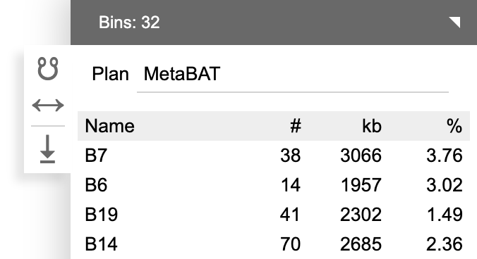
One may create a binning plan from de novo or load an existing one from a categorical field. Each category represents a bin. The name, number of contigs (#), total length of contigs (kb) and the relative abundance (calculated as length x coverage, then normalized against the entire assembly) are displayed.
When a binning plan is modified (added/removed bins, added/removed contigs to/from bins, renamed bins, entered a new plan name, etc.), a Save button will show up. Click it to save the binning plan as a categorical field.
Alternatively, click the ⇥ button in the toolbar to export the binning plan to a text file. The format will be a mapping of bin names to member contig IDs.
The table below the binning plan name displays a list of bins in the plan. Click a bin to select it. The contigs in this bin will be selected in the same time and their properties will be summarized.
Click the bin again to edit its name. Press Enter when done. Hold Shift and click to select multiple bins.
The toolbar next to the bin table provides a few utilities. Click + to create an empty new bin. Click − to delete the selected bin(s), Click ∪ to merge multiple bins.
Press Space to create a new bin from selected contigs. If no binning plan is currently loaded, the program will create a new plan. This is perhaps the easiest way to start de novo binning using the program.
Press . to add selected contigs to the select bin. Press , to remove selected contigs from the selected bin. Press / to update (replace) the selected bin with selected contigs.
These functions can also be found in the toolbar next to the summary table.
BinaRena can evaluate the confidence of binning by calculating the silhouette coefficient. Specifically, a silhouette coefficient measures how similar a contig is to other contigs in the same bin, as in contrast to contigs in other bins. It ranges from -1 (worst) to 1 (best).
One may click the ☋ button in the toolbar next to the binning plan to open the "silhouette coefficient" window. It allows the user to select variables to be included in the calculation.
- Note: Only select variables that are presumably homogeneous in each bin (e.g., GC%, coverage, k-mer frequency). Don't select those that aren't (e.g., length of contig).
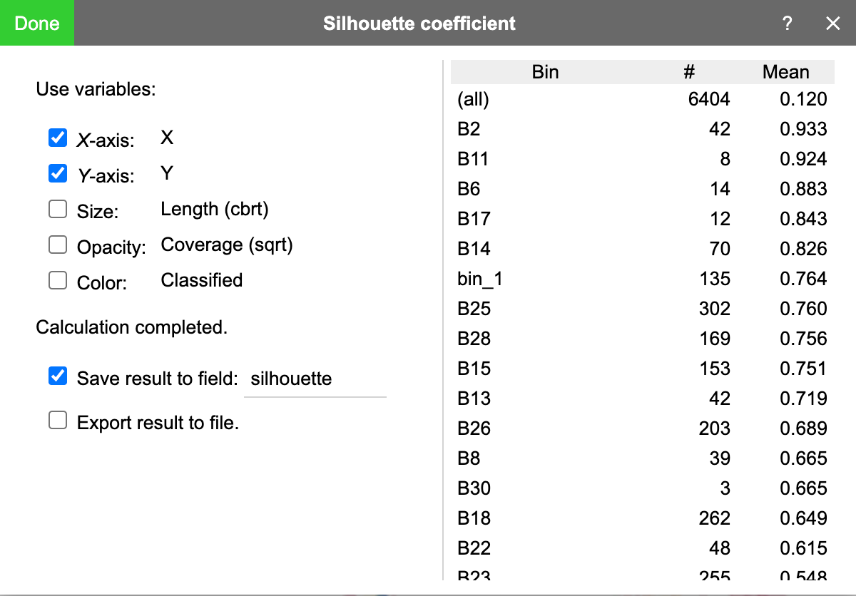
Then click the "calculate" button to start calculation. When done, the mean silhouette coefficient of each bin and all bins will be displayed in a table.
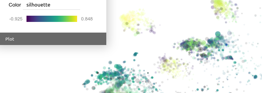
Before pressing "done", one may check "save result to field" to save the calculated silhouette coefficient to a categorical field. BinaRena will automatically color the contigs using these values, from which one can immediately see which bins are of high overall confidences and which contigs are confidently belonging to their bins. This can guide the subsequent binning efforts.
One may also check "export result to file" to save the results (contig IDs, bin assignments and silhouette coefficients) to a TSV file.
- Be warned not to over-interpret silhouette coefficient. It is a widely-used metric for cluster analysis evaluation. However, other biological factors may also be important in the task of binning.
BinaRena compares two binning plans by calculating the adjusted Rand index (ARI), which measures the consistency between two grouping scenarios of the same dataset. Higher is better. Two identical plans have ARI = 1. Two random plans will have an ARI close to 0.
One may click the ↔ button in the toolbar next to the binning plan, then select a categorical field (another binning plan) to perform this calculation. It is fast. The result will be displayed in a floating message box.
Do old browsers support BinaRena?
BinaRena is written in JavaScript, using mordern language standards including ES6 and above. Mordern browsers shouldn't have problems as they normally auto-update to meet the latest standards. However, very outdated browsers such as Internet Explorer may not support BinaRena.
Does BinaRena expose my data to a remote server?
The standalone BinaRena program is a client-end webpage that runs in your browser. Theoretically and technically, it cannot communicate with a web server. There is no risk with regard to the confidentiality of your data.
The live demo hosted by GitHub Pages can communicate with the GitHub repository, and the only thing it does is to retrieve the sample dataset from the repository directory. It does not perform any other communication.
How to precisely control the size of the plot?
Drag to resize the browser window. The plot will be resized along with it, during which its width and height (in unit of pixel) will be displayed in a floating message box.
Where are the color palettes in BinaRena from?
Most of these color palettes were adopted from Matplotlib, which have been widely utilized in Python data science. The default categorical palette "QIIME" was adopted from the EMPeror viewer of the microbiome data analysis package QIIME 2.
Can I customize the color palettes?
Not from the GUI. But look into static/js/resource.js and you know what to do.
In the exported SVG image, some data points are covered by the legends. Can I move the legends outside the plot?
The data points are covered, but they are not missing. One can open the SVG file in a vector image editor such as Inkscape, and move the legends away from the plot area. The covered elements will be revealed.
Can I customize the appearance of the exported SVG image?
The GUI doesn't provide much control. However, pro users can look into (static/js/svg.js). On top of the function renderSVG there are multiple customizable parameters.
How does BinaRena perform data ranking?
BinaRena sorts numeric values from small to large and assign them ranks 1, 2, 3... If there are ties, all numbers in a tie will receive the average rank of them. This behavior is consistent with the default behavior of SciPy's rankdata function.
How exactly does BinaRena calculate silhouette coefficients?
The silhouette coefficient calculation algorithm in BinaRena was implemented in reference to Scikit-learn's silhouette_score function to achieve compatible results. Prior to this final step, several operations are involved for data preprocessing:
The contigs are filtered to exclude those 1) that are not in any bin, 2) that are currently masked, 3) that have invalid values in any of the variables after transformation. The remaining data are subject to min-max scaling (consistent with the default behavior of Scikit-learn's MinMaxScaler) such that each variable is within the range of [0, 1]. Then, the pairwise Euclidean distances between contigs are calculated using the scaled variables. Finally, the silhouette coefficients were calculated.
One can monitor the process and intermediates using the browser's console.
Why does the program stall / crash during silhouette coefficient calculation?
Calculation of silhouette coefficients requires the calculation of a Euclidean distance matrix among all contigs. This is a computationally expensive operation. Runtime and memory consumption quickly build up as the dataset expands (O(n2)).
However, with a typical computer, it shouldn't take more than a few minutes even with tens of thousands of contigs. Just be bit patient before killing the browser tab.
- Note: Chrome and Edge have a mechanism to limit memory consumption per tab, hence blocking this function from handling more than some ten thousand of contigs. Firefox and Safari do not have this limitation.
When compute is an issue, it is recommended to filter down the dataset (e.g., removing short and shallow contigs) to make the calculation smooth.
Please forward any questions to the project leader: Dr. Qiyun Zhu (qiyunzhu@gmail.com).

