Camera and LIDAR Calibration and Visualization in ROS

Setting up ROS in vagrant

$ vagrant init shadowrobot/ros-indigo-desktop-trusty64

Open Vagrantfile in editor
- uncomment/edit these lines:

  config.vm.provider "virtualbox" do |vb|
  #   # Display the VirtualBox GUI when booting the machine
    vb.gui = true
  #
  #   # Customize the amount of memory on the VM:
    vb.memory = "2048"
  end

$ vagrant up

Wait for box to download and provision
When gui boots, open Terminal

$ sudo apt-get update
$ sudo apt-get upgrade

Inspecting bag file

Move '.bag' file to the same folder as Vagrantfile

Inside VM:

$ rosbag info 2016-11-22-14-32-13_test.bag

Sample output:

path:        2016-11-22-14-32-13_test.bag
version:     2.0
duration:    1:53s (113s)
start:       Nov 22 2016 16:32:14.41 (1479853934.41)
end:         Nov 22 2016 16:34:07.88 (1479854047.88)
size:        3.1 GB
messages:    5975
compression: none [1233/1233 chunks]
types:       sensor_msgs/CameraInfo  [c9a58c1b0b154e0e6da7578cb991d214]
             sensor_msgs/Image       [060021388200f6f0f447d0fcd9c64743]
             sensor_msgs/PointCloud2 [1158d486dd51d683ce2f1be655c3c181]
topics:      /sensors/camera/camera_info   2500 msgs    : sensor_msgs/CameraInfo 
             /sensors/camera/image_color   1206 msgs    : sensor_msgs/Image      
             /sensors/velodyne_points      2269 msgs    : sensor_msgs/PointCloud2

Playing bag file

Inside VM:

$ rosbag play 2016-11-22-14-32-13_test.bag

To play at slower speed, e.g. 50%:

$ rosbag play -r 0.5 2016-11-22-14-32-13_test.bag

Note: This may be required depending on the speed of the host PC.

Task #1: Camera Calibration

Note: The checker board pattern used 5 x 7 corners and size of each square 5 cm.

Automatic Calibration using `cameracalibrator.py`

Following tutorial from ROS Wiki

$ rosdep install camera_calibration
$ rosmake camera_calibration

Inside VM:

$ rosrun camera_calibration cameracalibrator.py --size=5x7 --square=0.050 image:=/sensors/camera/image_color camera:=/sensors/camera/camera_info  --no-service-check

Bag file was played back at 50% speed to allow cameracalibrator.py to collect enough images to cover the X, Y, Size, and Skew parameter spaces.
24 images were collected

Results

image_width: 964
image_height: 724
camera_name: narrow_stereo
camera_matrix:
  rows: 3
  cols: 3
  data: [483.306502, 0.000000, 456.712456, 0.000000, 482.958638, 366.254245, 0.000000, 0.000000, 1.000000]
distortion_model: plumb_bob
distortion_coefficients:
  rows: 1
  cols: 5
  data: [-0.197847, 0.065563, 0.003166, -0.000043, 0.000000]
rectification_matrix:
  rows: 3
  cols: 3
  data: [1.000000, 0.000000, 0.000000, 0.000000, 1.000000, 0.000000, 0.000000, 0.000000, 1.000000]
projection_matrix:
  rows: 3
  cols: 4
  data: [409.833832, 0.000000, 456.584871, 0.000000, 0.000000, 410.319702, 370.492937, 0.000000, 0.000000, 0.000000, 1.000000, 0.000000]

Manual Calibration

Use image_view to collect images. Right click to save screenshot.

$ rosrun image_view image_view image:=/sensors/camera/image_color

30 images were saved as frame0000.jpg to frame0029.jpg.
part1.py was created to perform calibration using these images.

import cv2
from camera_calibration.calibrator import MonoCalibrator, ChessboardInfo

numImages = 30

images = [ cv2.imread( '../Images/frame{:04d}.jpg'.format( i ) ) for i in range( numImages ) ]

board = ChessboardInfo()
board.n_cols = 7
board.n_rows = 5
board.dim = 0.050

mc = MonoCalibrator( [ board ], cv2.CALIB_FIX_K3 )
mc.cal( images )
print( mc.as_message() )

mc.do_save()

Run part1.py

$ cd scripts
$ python part1.py

Results

image_width: 964
image_height: 724
camera_name: narrow_stereo/left
camera_matrix:
  rows: 3
  cols: 3
  data: [485.763466, 0.000000, 457.009020, 0.000000, 485.242603, 369.066006, 0.000000, 0.000000, 1.000000]
distortion_model: plumb_bob
distortion_coefficients:
  rows: 1
  cols: 5
  data: [-0.196038, 0.062400, 0.002179, 0.000358, 0.000000]
rectification_matrix:
  rows: 3
  cols: 3
  data: [1.000000, 0.000000, 0.000000, 0.000000, 1.000000, 0.000000, 0.000000, 0.000000, 1.000000]
projection_matrix:
  rows: 3
  cols: 4
  data: [419.118439, 0.000000, 460.511129, 0.000000, 0.000000, 432.627686, 372.659509, 0.000000, 0.000000, 0.000000, 1.000000, 0.000000]

Rectifying images

Adding calibration information to bag files

Install bag_tools

$ sudo apt-get install ros-indigo-bag-tools

Note: rosrun couldn't find change_camera_info.py, but it was in /opt/ros/indigo/lib/python2.7/dist-packages/bag_tools so it was copied into the scripts directory.

Create new bagfiles with calibration data

For cameracalibrator.py output:

python change_camera_info.py ../2016-11-22-14-32-13_test.orig.bag ../2016-11-22-14-32-13_test.cameracalibrator.bag /sensors/camera/camera_info=../Results/calibrationdata_cameracalibrator.yaml

For part1.py output:

python change_camera_info.py ../2016-11-22-14-32-13_test.orig.bag ../2016-11-22-14-32-13_test.part1.bag /sensors/camera/camera_info=../Results/calibrationdata_part1.yaml

Create launch file for recording rectified image

image_proc was used to rectify the image based on the new calibration information.

Three .launch files were created to record three different results: original image, rectified image using manual calibration data, and rectified image using automatic calibration data.

The files for the rectified images were similar with the only difference being which bagfile was passed to rosbag. The image_proc node was removed when recording the original image.

<launch>
	<node name="rosbag" pkg="rosbag" type="play" args="/vagrant/2016-11-22-14-32-13_test.cameracalibrator.bag"/>
	<node name="image_proc" pkg="image_proc" type="image_proc" respawn="false" ns="/sensors/camera">
		<remap from="image_raw" to="image_color"/>
	</node>
	<node name="rect_video_recorder" pkg="image_view" type="video_recorder" respawn="false">
		<remap from="image" to="/sensors/camera/image_rect_color"/>
	</node>
</launch>

By default, video_recorder creates output.avi in /home/ros/.ros. After running each launch file, the resulting output.avi was renamed and copied to the ../Results directory.

Compare Calibration Results

The three videos were placed side by side using ffmpeg in order to more easily compare the results of the image rectification.

$ ffmpeg -i calibration-original.avi -i calibration-part1.avi -i calibration-cameracalibrator.avi -filter_complex '[0:v]pad=iw*3:ih[int];[int][1:v]overlay=W/3:0[int2];[int2][2:v]overlay=2*W/3:0,drawtext=fontsize=60:fontcolor=#095C8D:fontfile=/usr/share/fonts/truetype/freefont/FreeSans.ttf:text='Original':x=W/6+100:y=25,drawtext=fontsize=60:fontcolor=#095C8D:fontfile=/usr/share/fonts/truetype/freefont/FreeSans.ttf:text='Manual':x=3*W/6+100:y=25,drawtext=fontsize=60:fontcolor=#095C8D:fontfile=/usr/share/fonts/truetype/freefont/FreeSans.ttf:text='Automated':x=5*W/6+100:y=25[vid]' -map [vid] -c:v libx264 -crf 23 -preset veryfast part1-combined.mp4

The resulting video can be found here.

Note: The videos are not synchronized, but they're close enough to see the results of the comparison.

The image below shows a representative capture of the calibrations. The original image is on the left, and the rectified images from the manual and automatic calibrations are in the middle and right, respectively. As you can see, the manual calibration does not correct the radial distortion at the far edges of the image; however, both calibrations show a rectified checker board in the center of the image. In typical use cases, both calibrations should be adequate.

Task #2: LIDAR to Image Calibration

Running Image / LIDAR calibration

A ROS package was created to hold scripts used to run calibration. To use them, first add scripts folder to ROS_PACKAGE_PATH

$ export ROS_PACKAGE_PATH=/vagrant/scripts:$ROS_PACKAGE_PATH

A launch file was created to start calibration

$ roslaunch launch/part2-cameralidar-calibration.launch

<launch>
	<node name="rosbag" pkg="rosbag" type="play" args="/vagrant/2016-11-22-14-32-13_test.part1.bag"/>
	<node name="lidar_image_calibration" pkg="lidar_image_calibration" type="lidar_image_calibration.py" args="/vagrant/data/lidar_image_calibration_data.json Images/lidar_calibration_frame.jpg /vagrant/Results/Images/lidar_calibration_output.jpg " output="screen">
		<remap from="camera" to="/sensors/camera/camera_info"/>
	</node>
</launch>

The script scripts/lidar_image_calibration/lidar_image_calibration.py requires a .json file containing point correspondences between 3D Points and 2D image coordinates. The point correspondences used to generate the results below can be found in data/lidar_image_calibration_data.json. Optional parameters can be included to generate an image using the expected and generated image coordinates for the provided 3D points.

{
	"points": [ 
		[ 1.568, 0.159, -0.082, 1.0 ], // top left corner of grid
		[ 1.733, 0.194, -0.403, 1.0 ], // bottom left corner of grid
		[ 1.595, -0.375, -0.378, 1.0 ], // bottom right corner of grid
		[ 1.542, -0.379, -0.083, 1.0 ], // top right corner of grid
		[ 1.729, -0.173, 0.152, 1.0 ], // middle of face
		[ 3.276, 0.876, -0.178, 1.0 ] // corner of static object
	],
	"uvs": [
		[ 309, 315 ],
		[ 304, 433 ],
		[ 491, 436 ],
		[ 490, 321 ],
		[ 426, 286 ],
		[ 253, 401 ]
	],
	"initialTransform": [ 0.0, 0.0, 0.0, 0.0, 0.0, 0.0 ],
	"bounds": [
		[ -5, 5 ],
		[ -5, 5 ],
		[ -5, 5 ],
		[ 0, 6.28318530718 ], // 2 * pi
		[ 0, 6.28318530718 ], // 2 * pi
		[ 0, 6.28318530718 ] // 2 * pi
	]
}

How it works

The calibration script relies on the scipy.optimize.minimize function to find the translation and rotation between the camera frame and LIDAR frame. minimize can perform bounded optimization to limit the state parameters. The translation along each axis is limited to ± 5.0 meters. The rotation angles are limited between 0 and 360 degrees (2 pi radians).

The cost function to be minimized is the sum of the magnitudes of the error between expected UV coordinates and those obtained by the state parameters at each step of the optimization.

Some initial state vectors, including [ 0, 0, 0, 0, 0, 0 ], has a positive gradient in the neighborhood surrounding it. This results in unsuccessful optimization. To counteract this, a new initial state vector is picked randomly within the bounds of each parameter. In order to find a minima closer to the unknown global minimum, new initial state vectors are also randomly picked until a successful optimization results in an error of less than 50 pixels.

Creating the composite LIDAR image

Once the optimized state parameters are found by the previous step, the state vector can be added to the static_transform_provider node inside Launch/part2-cameralidar.launch.

<launch>
	<param name="use_sim_time" value="true" />
	<node name="rosbag" pkg="rosbag" type="play" args="-r 0.25 --clock /vagrant/2016-11-22-14-32-13_test.part1.bag"/>
	<node name="image_proc" pkg="image_proc" type="image_proc" respawn="false" ns="/sensors/camera">
		<remap from="image_raw" to="image_color"/>
	</node>
	<node name="tf" pkg="tf" type="static_transform_publisher" args="-0.05937507 -0.48187289 -0.26464405  5.41868013  4.49854285 2.46979746 world velodyne 10"/>
	<node name="lidar_image_calibration" pkg="lidar_image_calibration" type="lidar_image.py" args="">
		<remap from="image" to="/sensors/camera/image_rect_color"/>
		<remap from="image_lidar" to="/sensors/camera/image_lidar"/>
		<remap from="camera" to="/sensors/camera/camera_info"/>
		<remap from="velodyne" to="/sensors/velodyne_points"/>
	</node>
	<!--<node name="image_view" pkg="image_view" type="image_view" args="">
		<remap from="image" to="/sensors/camera/image_lidar"/>
	</node>-->
	<node name="rect_video_recorder" pkg="image_view" type="video_recorder" respawn="false">
		<remap from="image" to="/sensors/camera/image_lidar"/>
	</node>
</launch>

This launch file provides the option to view the composite image in real-time through image_view or to record a video containing the images for the entire data stream.

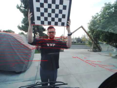
The image below shows an example of the composite image.

How it works

lidar_image.py subscribes to the following data sources:

The rectified camera image: /sensors/camera/image_rect_color
The calibration transform: /world/velodyne
The camera calibration information for projecting the LIDAR points: /sensors/camera/camera_info
The Velodyne data scan: /sensors/velodyne_points

As each LIDAR scan is received, the scan data is unpacked from the message structure using struct.unpack. Each scan point contains the x, y, and z coordinates in meters, and the intensity of the reflected laser beam.

formatString = 'ffff'
if data.is_bigendian:
  formatString = '>' + formatString
else:
  formatString = '<' + formatString

points = []
for index in range( 0, len( data.data ), 16 ):
  points.append( struct.unpack( formatString, data.data[ index:index + 16 ] ) )

This is needed because there are not officially supported Python libraries for Point Cloud Library. The python_pcl package has been created and is available here. While this module was compiled and tested, the simplicity of unpacking the structure manually was chosen over importing an external module.

As each image is received, cv_bridge is used to convert the ROS Image sensor message to an OpenCV compatible format.

The /world/velodyne transform is obtained each frame. This proved useful during an attempt at manual calibration. This is converted into an affine transformation matrix containing the rotation and translation between frames.

Each point of the laser scan was then transformed into the camera frame. Points that are more than 4.0 meters away from the camera were thrown out to aid in declutter the composite image. Points with negative z value were also thrown out as they represent scan points which are behind the camera's field of view.

A pin hole camera model was used to project the rotated 3D points into image coordinates. Red circles are rendered for each point which is projected inside the image bounds.

Results

Six points were picked for image calibration using rviz

Top left corner of calibration grid
Bottom left corner of calibration grid
Bottom right corner of calibration grid
Top right corner of calibration grid
The center of the face of the person holding the calibration grid
The corner of the static object on the left side of the image

The optimized transform obtained was:

# Position in meters, angles in radians
( offsetX, offsetY, offsetZ, yaw, pitch, roll ) = [ -0.05937507, -0.48187289, -0.26464405, 5.41868013, 4.49854285, 2.46979746 ]

# Angles in degrees
( yawDeg, pitchDeg, rollDeg ) = [ 310.4675019812, 257.7475192644, 141.5089707105 ]

The image below shows the expected image coordinates in blue and the points created by the optimized transform in red.

As you can see, the most error comes from the point on the face and the points on the right side of the calibration grid. However, the total error obtained is only about 35 pixels.

Using this transform, a video was created to show how well all of the LIDAR points in the bagfile align to the image. Because this code is running in a virtual machine and the LIDAR scans at a higher frequency, the image and LIDAR scans are not in sync; however, when the person in the image stops for a moment, you can see how well the calibration worked.

The resulting video can be found here.

Note: This video was sped up to 2x speed to account for the slower rate the bagfile was played.

$ ffmpeg -i Results/Videos/part2-lidar-image.avi -filter:v "setpts=0.5*PTS" -c:v libx264 -crf 23 -preset veryfast output.mp4

Task #3: RGB Point Cloud from LIDAR and Image Data

Instead of projecting the points onto an image, you can also project the image data onto the 3D point cloud using the same information.

The script scripts/lidar_image_calibration/lidar_rgb.py was created to transmit a new point cloud containing RGB data for each point which can be projected onto the image.

Each received image is stored for use when every point cloud is received. Each point in the cloud is read using pcl2.read_points( data ) instead of manually unpacking data as was done in lidar_image.py. pcl2.create_cloud was used to pack the point data ( 3D position, intensity, and RGB color ) into a PointCloud2 message for publishing.

Running the script

A launch file was created to run all of the required ROS nodes.

$ roslaunch launch/part3-rgbpointcloud.launch

<launch>
	<param name="use_sim_time" value="true" />
	<node name="rosbag" pkg="rosbag" type="play" args="-r 0.01 -s 73 --clock /vagrant/2016-11-22-14-32-13_test.part1.bag"/>
	<node name="image_proc" pkg="image_proc" type="image_proc" respawn="false" ns="/sensors/camera">
		<remap from="image_raw" to="image_color"/>
	</node>
	<node name="tf" pkg="tf" type="static_transform_publisher" args="-0.05937507 -0.48187289 -0.26464405  5.41868013  4.49854285 2.46979746 world camera 10"/>
	<node name="tf" pkg="tf" type="static_transform_publisher" args="0 0 0 0 0 0 world velodyne 10"/>
	<node name="lidar_rgb" pkg="lidar_image_calibration" type="lidar_rgb.py" args="">
		<remap from="image" to="/sensors/camera/image_rect_color"/>
		<remap from="camera" to="/sensors/camera/camera_info"/>
		<remap from="velodyne" to="/sensors/velodyne_points"/>
		<remap from="velodyne_rgb_points" to="/sensors/velodyne_rgb_points"/>
	</node>
</launch>

Two different transformation frames were created:

/world/camera: LIDAR to image calibration
/world/velodyne: Identity transform so that the data shows up better in rviz

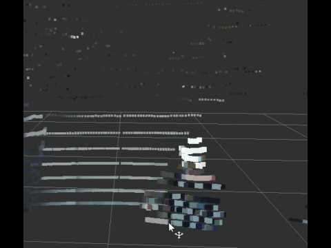
Results

Kazam was used to capture a short video of the RGB point cloud viewed inside of rviz. The results aren't great because there's a lot of computation involved, the images and point clouds are received at different frequencies, and testing was performed inside a virtual machine.

The resulting video can be found here.

Note: This video was sped up to 2x speed to account for the slower rate the bagfile was played.

$ ffmpeg -i Results/Videos/rgb_pointcloud.mp4 -filter:v "setpts=0.5*PTS" -c:v libx264 -crf 23 -preset veryfast Results/Videos/rgb_pointcloud.mp4

rgreid/ros-camera-lidar-calibration

Camera and LIDAR Calibration and Visualization in ROS

Setting up ROS in vagrant

Inspecting bag file

Playing bag file

Task #1: Camera Calibration

Automatic Calibration using cameracalibrator.py

Results

Manual Calibration

Results

Rectifying images

Adding calibration information to bag files

Create launch file for recording rectified image

Compare Calibration Results

Task #2: LIDAR to Image Calibration

Running Image / LIDAR calibration

How it works

Creating the composite LIDAR image

How it works

Results

Task #3: RGB Point Cloud from LIDAR and Image Data

Running the script

Results

Automatic Calibration using `cameracalibrator.py`