The goals / steps of this project are the following:
- Compute the camera calibration matrix and distortion coefficients given a set of chessboard images.
- Apply a distortion correction to raw images.
- Use color transforms, gradients, etc., to create a thresholded binary image.
- Apply a perspective transform to rectify binary image ("birds-eye view").
- Detect lane pixels and fit to find the lane boundary.
- Determine the curvature of the lane and vehicle position with respect to center.
- Warp the detected lane boundaries back onto the original image.
- Output visual display of the lane boundaries and numerical estimation of lane curvature and vehicle position.
The images for camera calibration are stored in the folder called camera_cal. The images in test_images are for testing your pipeline on single frames. If you want to extract more test images from the videos, you can simply use an image writing method like cv2.imwrite(), i.e., you can read the video in frame by frame as usual, and for frames you want to save for later you can write to an image file.
To help the reviewer examine your work, please save examples of the output from each stage of your pipeline in the folder called output_images, and include a description in your writeup for the project of what each image shows. The video called project_video.mp4 is the video your pipeline should work well on.
The challenge_video.mp4 video is an extra (and optional) challenge for you if you want to test your pipeline under somewhat trickier conditions. The harder_challenge.mp4 video is another optional challenge and is brutal!
Advanced_LaneFinding_Pipeline.py- Contains the class that essentially performs the pipeline.
preprocessing_frames.py- contains the class that calculates the color and thresholded gradients.
Advanced_Lane_Finding_Workouts.ipynb- Contains the workouts, experiments done.
- Experiments - camera calibration, perspective transforms, thresholded gradients and color gradients interactive exploration.
Advanced_LF_Class_Pipeline.ipynb- contains the pipeline detector of advanced lane lines.
Advanced Lane Finding Project [//]: # (Image References)
Rubric Points
Here I will consider the rubric points individually and describe how I addressed each point in my implementation.
1. Provide a Writeup / README that includes all the rubric points and how you addressed each one. You can submit your writeup as markdown or pdf. Here is a template writeup for this project you can use as a guide and a starting point.
You're reading it!
1. Briefly state how you computed the camera matrix and distortion coefficients. Provide an example of a distortion corrected calibration image.
The code for this step is contained in the first code cell of the IPython notebook located in "./Advanced_Lane_Finding_Workouts.ipynb" ( in lines under the heading "Computing calibration matrix and distortion coefficients")
I start by preparing "object points", which will be the (x, y, z) coordinates of the chessboard corners in the world. Here I am assuming the chessboard is fixed on the (x, y) plane at z=0, such that the object points are the same for each calibration image. Thus, objp is just a replicated array of coordinates, and objpoints will be appended with a copy of it every time I successfully detect all chessboard corners in a test image.
I loaded the calibration chess pattern images, converted to grayscale. Then applied the cv2.findChessboardCorners()
function, supplied in with the columns=9 and rows=6 as its been clearly seen in the images.
imgpoints will be appended with the (x, y) pixel position of each of the corners in the image plane with each successful chessboard detection.
I then used the output objpoints and imgpoints to compute the camera calibration and distortion coefficients using the cv2.calibrateCamera() function. I applied this distortion correction to the test image using the cv2.undistort() function and also I had saved the calculated camera matrix, distortion coefficients in a pickle file for direct later application.
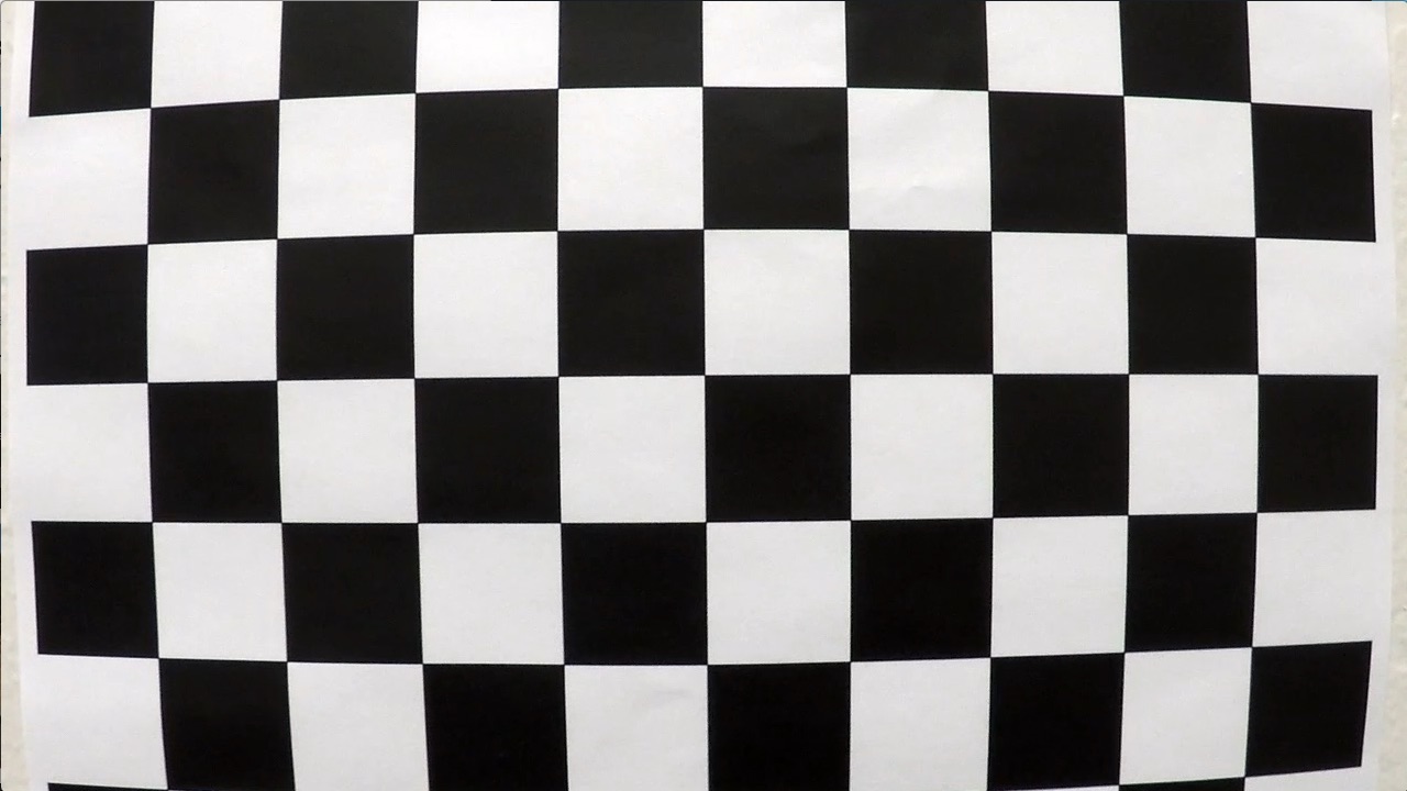
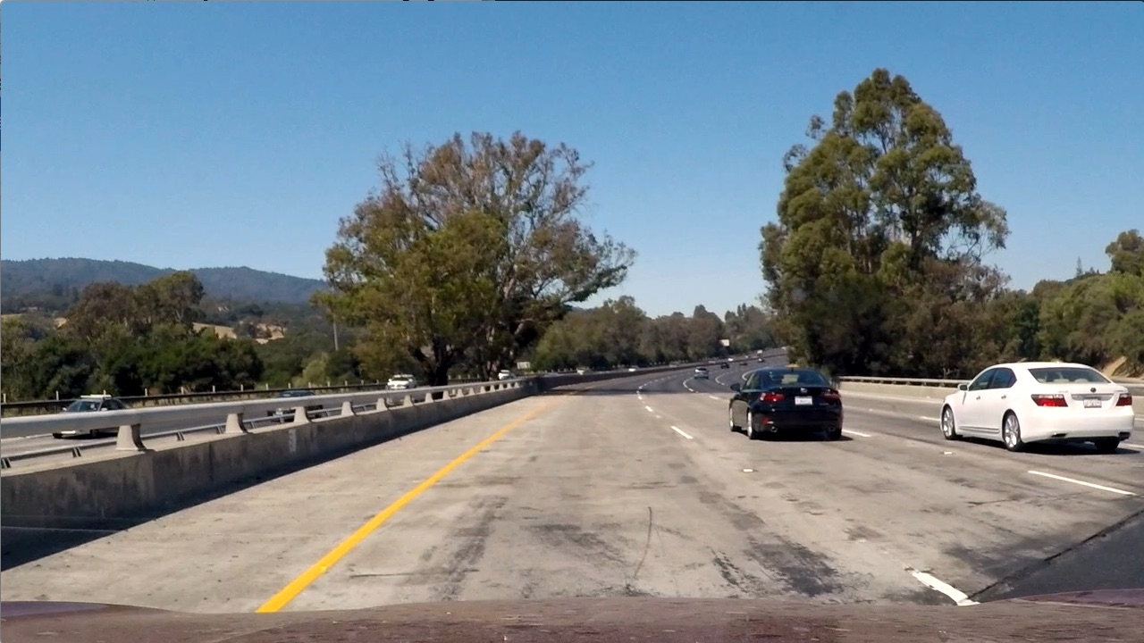
Distorted Image:
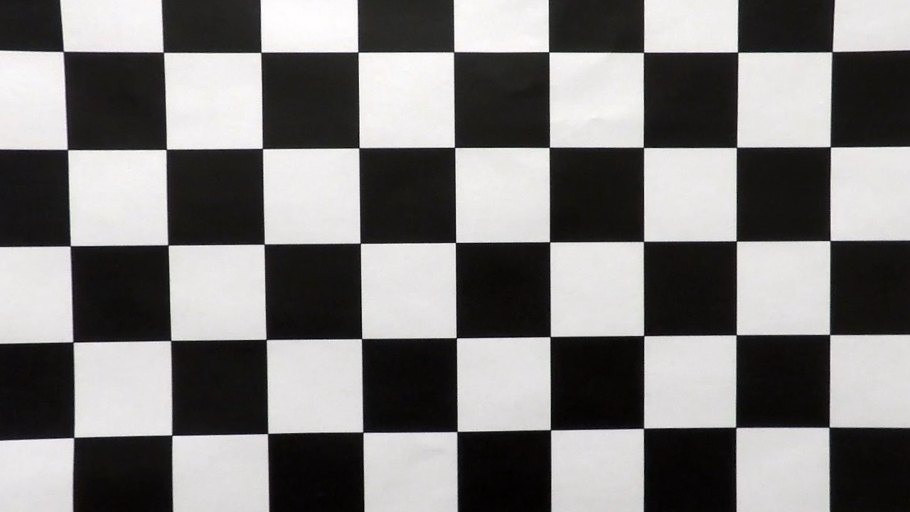
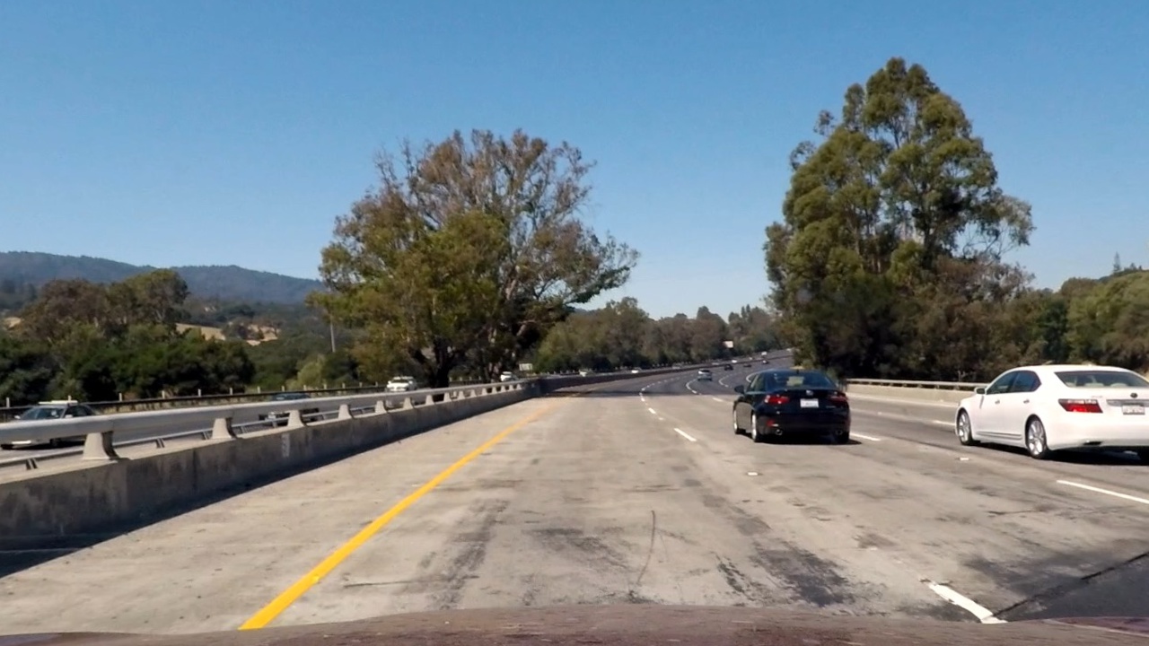
Here is an example of the corresponding Undistorted Image:
Please find the example of a distorted Image:
Please find the example of the distortion corrected corresponding image:
2. Describe how (and identify where in your code) you used color transforms, gradients or other methods to create a thresholded binary image. Provide an example of a binary image result.
I used a combination of color and gradient thresholds to generate a binary image (thresholding steps at lines 89 through 104 in Advanced_LaneFinding_Pipeline.py).
Steps:
- I had thresholded the gradients on the LAB color space on the L channel.
- I had used most of the code from udacity tutorial and snippets found online for the member functions
- For color gradients I had used the HLS color space as from my previous review I was informed about the prominent display of the yellow lanes in this space.
- So I extracted the yellow and white pixels the image by identifying the intervals at each channel.
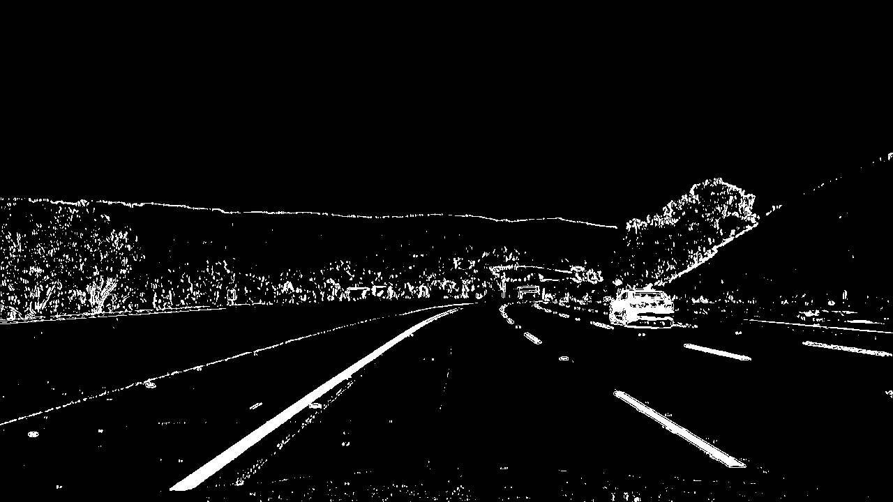
- Finally, combined the color gradients and the thresholded gradients in the output binary image displayed below,
(Please Note: Identifying the parameters took a long time. I found a easier way to achieve this by making use of the decorator function(@interact). You can find it in the notebook Advanced_Lane_Finding_Workouts.ipynb)
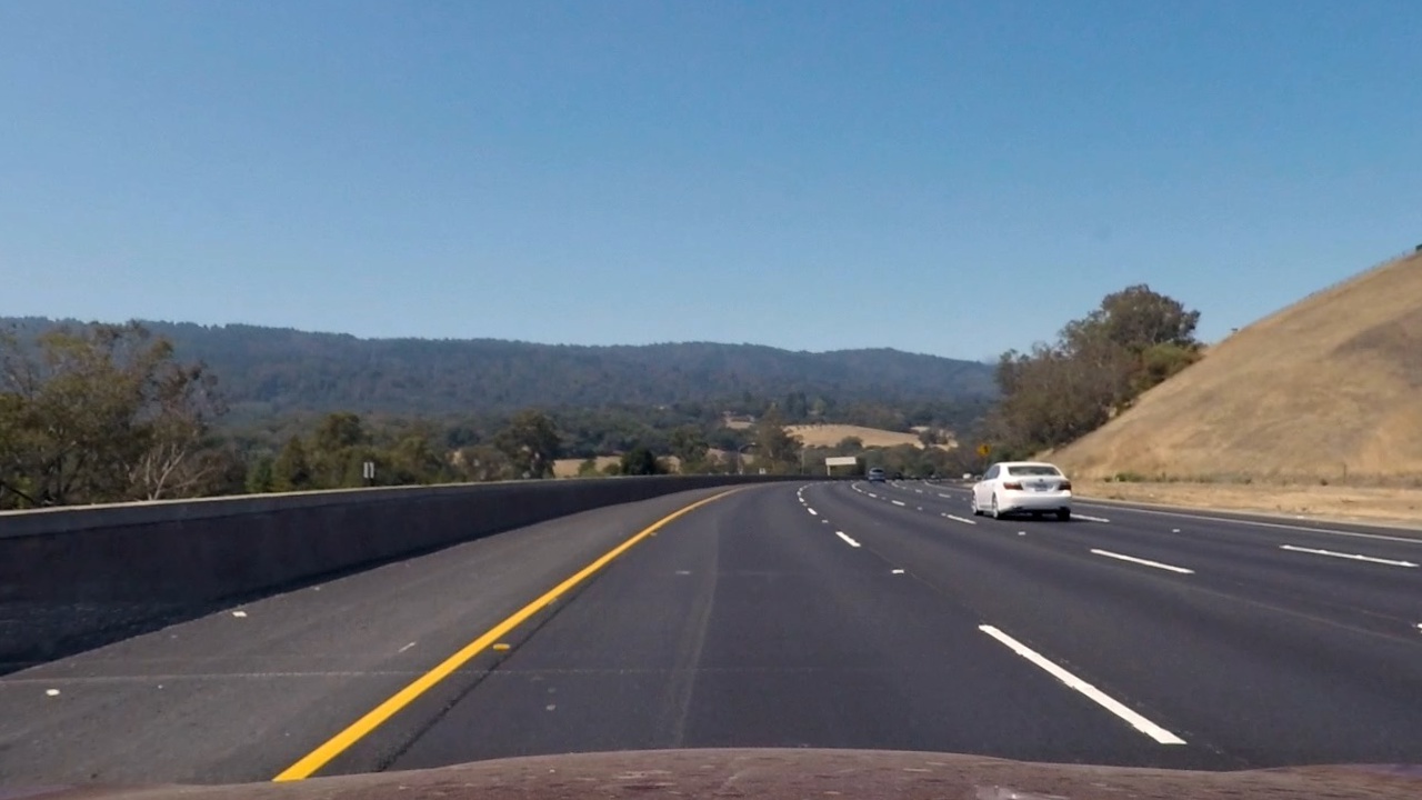
Input Image:
Here's an example of my output for this step. (note: this is not actually from one of the test images)
3. Describe how (and identify where in your code) you performed a perspective transform and provide an example of a transformed image.
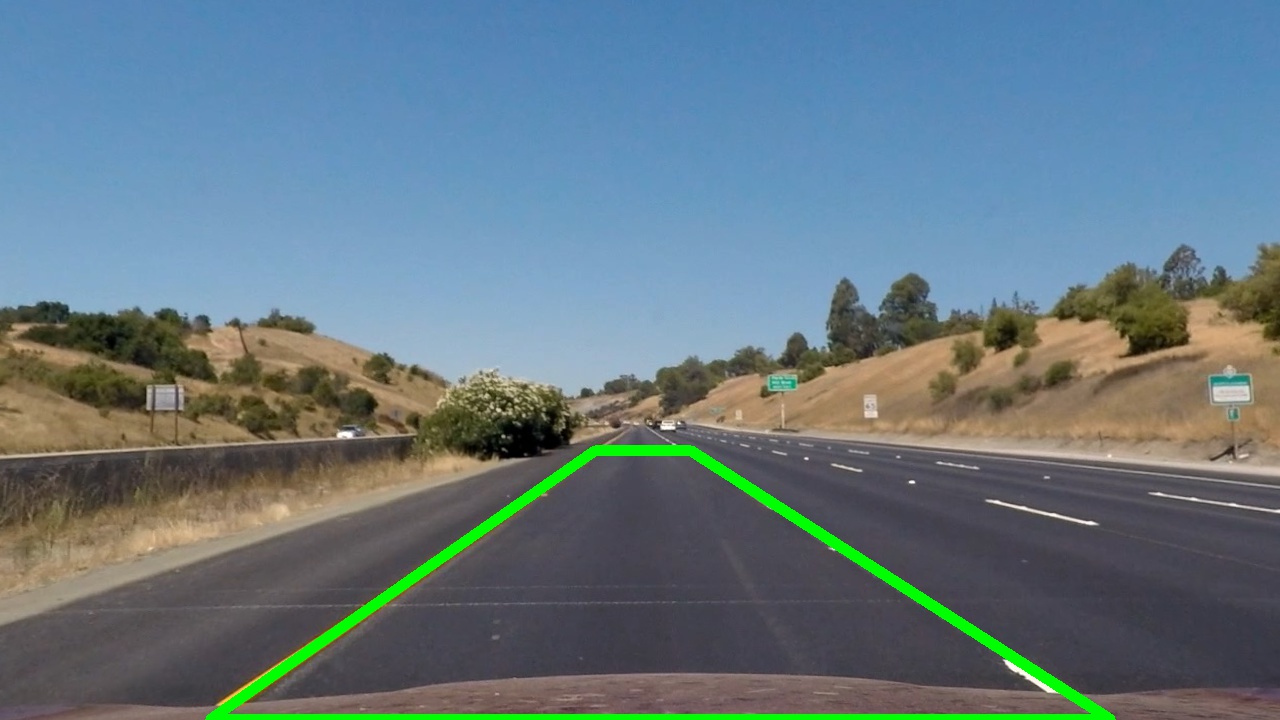
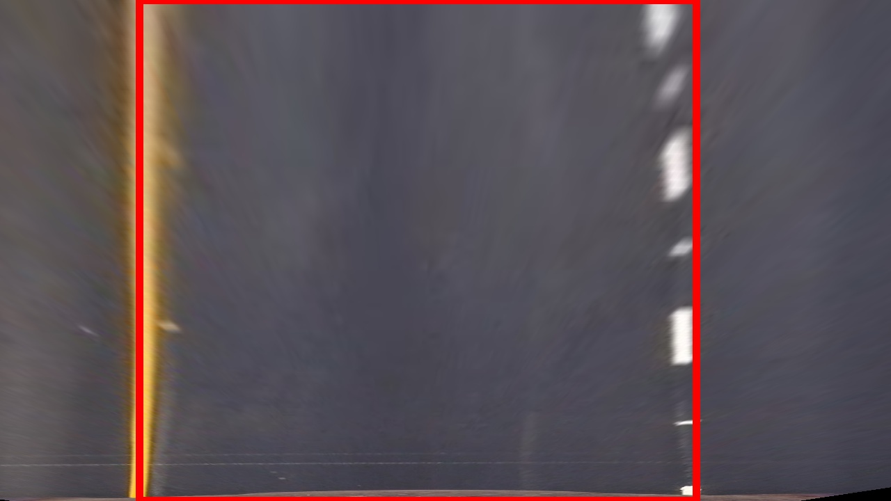
The code for my perspective transform includes a function called perspective_transform(img, src, dst), which can be found at 18th code cell in the notebook Advanced_Lane_Finding_Workouts.ipynb). The perspective_transform() function takes as inputs an image (img), as well as source (src) and destination (dst) points. I chose the hardcode the source and destination points in the following manner:
src = np.float32(
    [[210,719],
    [595,450],
    [690,450],
    [1110, 719]])
dst = np.float32(
    [[200, 719],
    [200, 0],
    [1000, 0],
    [1000, 719]])
This resulted in the following source and destination points:
| Source | Destination |
|---|---|
| 210, 719 | 200, 719 |
| 595, 450 | 200, 0 |
| 690, 450 | 1000, 0 |
| 1110, 719 | 1000, 719 |
The input image with Region Of Interest is below:
I verified that my perspective transform was working as expected by drawing the src and dst points onto a test image and its warped counterpart to verify that the lines appear parallel in the warped image.
4. Describe how (and identify where in your code) you identified lane-line pixels and fit their positions with a polynomial?
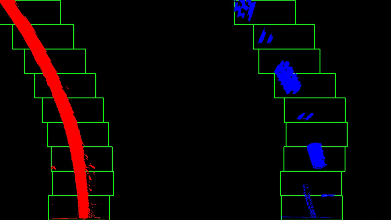
Steps :
- Apply the processed thresholded image with a perspective transform.
- Find the histogram peakpoints on the bottom-half of the image as the lanes are vertical to the vehicle.
- Calculate the nwindows per frame and the nonzero pixels in the image.
- split at the center for the left and right lane bases.
- calculate the non-zeros positives in each window and proceed to the top window by sliding the windows based on the non-zero pixel spread.
- With the obtained positive indices, we obtain the nonzero pixels that enables the calculation of the polynomial fits.
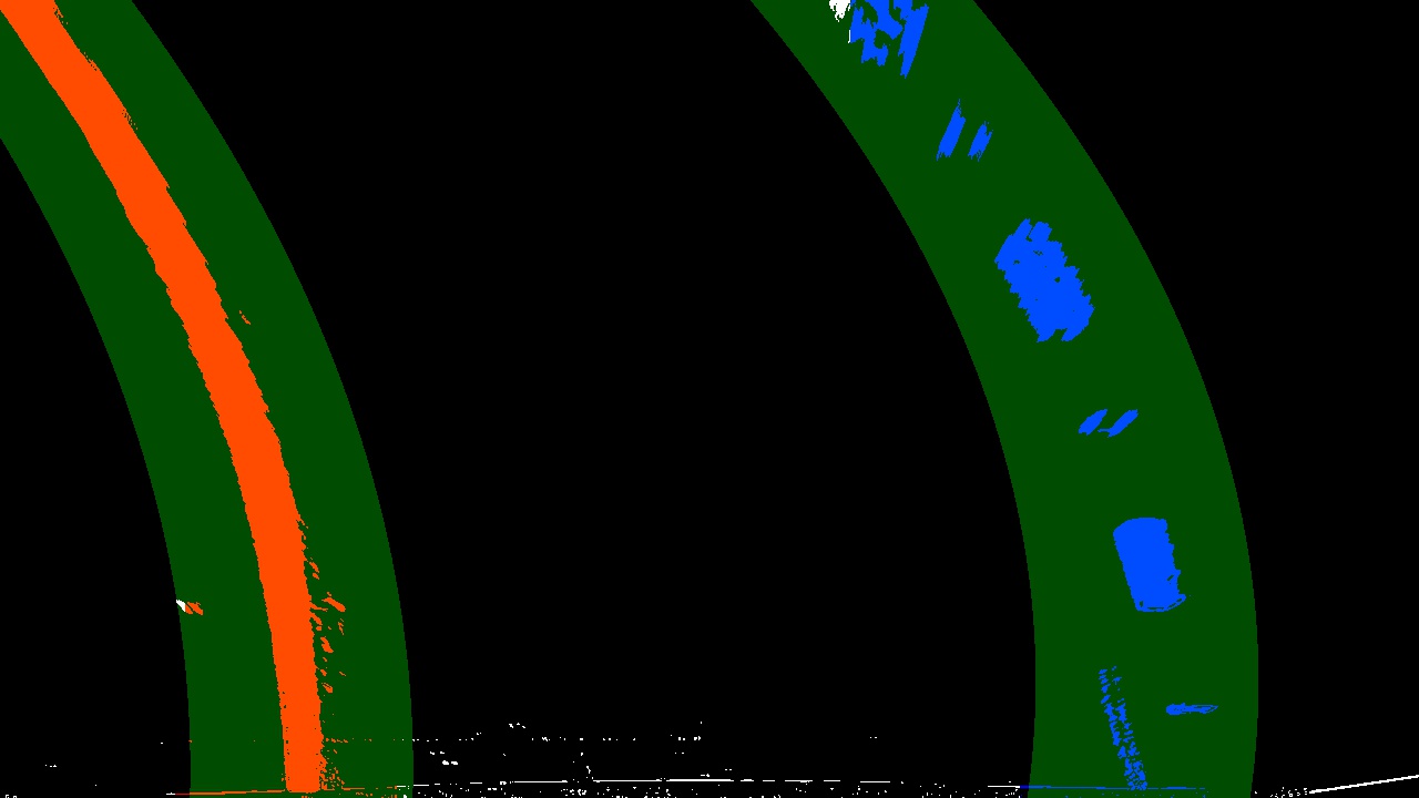
Below the stages are depicted;
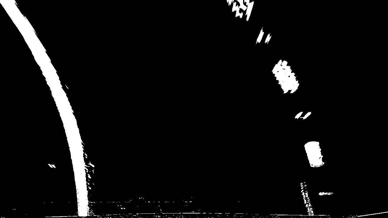
Input Warped Thresholded Image:
Fit Lanes and Bounded Image:
Bounded Region Image:
5. Describe how (and identify where in your code) you calculated the radius of curvature of the lane and the position of the vehicle with respect to center.
I did this in lines 238 through 268 in my code in Advanced_LaneFinding_Pipeline.py
Radii of Curvature calculation formula:
r = (1 + (first_derivative)**2)**1.5 / abs(second_derivative)- Using the formula, I had calculated the radius of curvature of the both left and right lanes respectively.
center_offset_img_space = (((left_fit[0] * y_eval ** 2 + left_fit[1] * y_eval + left_fit[2]) +
                                    (right_fit[0] * y_eval ** 2 + right_fit[1] * y_eval + right_fit[
2])) / 2) - lane_center- Difference between the Average of the lane polynomial coefficients and the lane center.
- Based on the central offset sign value, the alignment of the vehicles position identified.
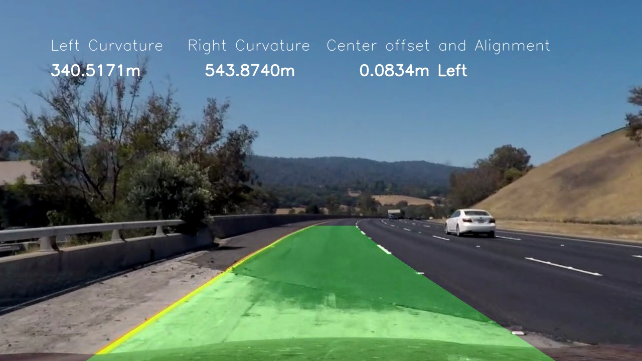
6. Provide an example image of your result plotted back down onto the road such that the lane area is identified clearly.
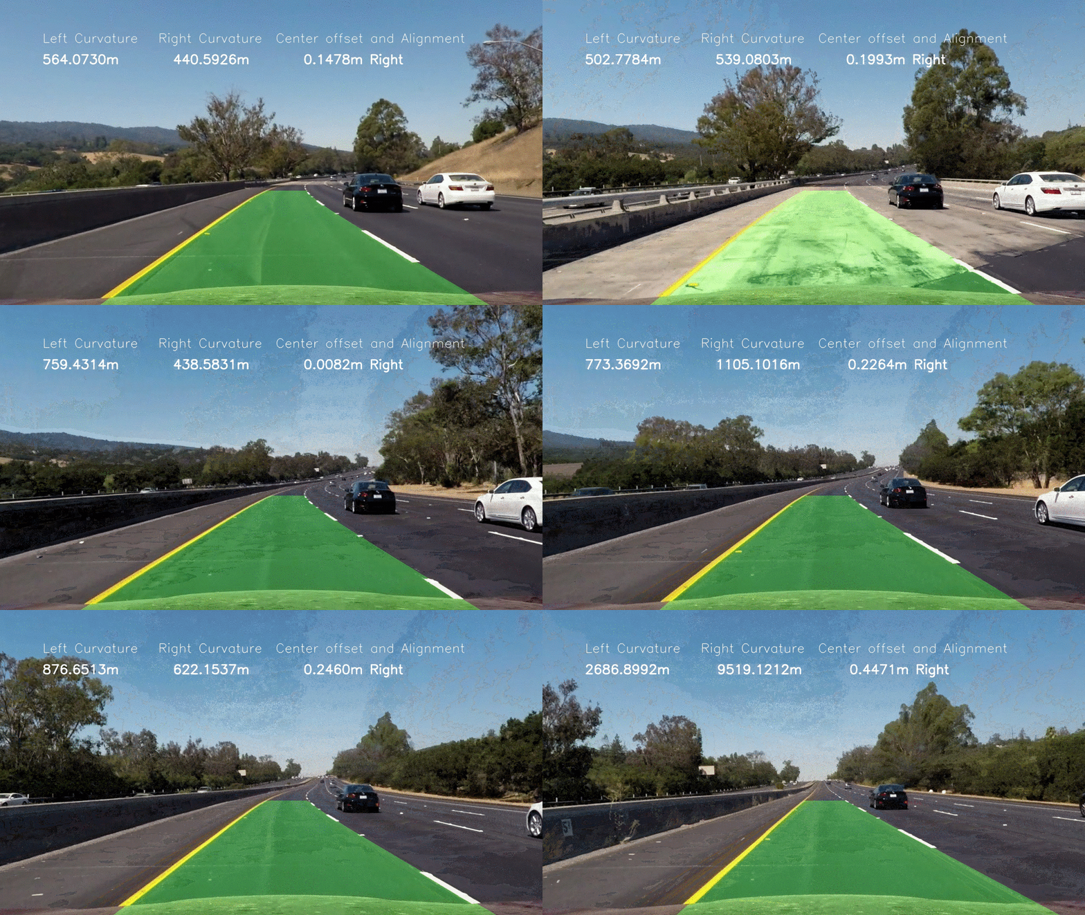
I implemented this step in lines 270 through 318 in my code in Advanced_LaneFinding_Pipeline.py.in the functions draw_lane_area(), draw_lane_curvature_text(). Here is an example of my result on a test image:
1. Provide a link to your final video output. Your pipeline should perform reasonably well on the entire project video (wobbly lines are ok but no catastrophic failures that would cause the car to drive off the road!).
 Here's a link to my video result
1. Briefly discuss any problems / issues you faced in your implementation of this project. Where will your pipeline likely fail? What could you do to make it more robust?
Challenges Faced:
- Obtaining the parameters i.e., the tuning part for the thresholding consumed time, also exploring different color spaces. Thanks some reference online I had an initial approx value for the params.
- The algorithm works fine with the supplied task video but there are minor discrepencies are still seen, when the vehicle enters different shades of road. It was minimized.
Pipeline failure:
- The pipeline fails for the challenge video and harder challenge one. The polynomials gets skewed.
- In the
challenge video, the lanes are not detected properly meaning, it detects the shadow edge as lanes and not the actual lanes - See below:
- Similar results on the
harder challenge videoas well. It fails to detect the lanes.
I believe that the pipeline can be improved to make it robust with better parameters. However the pipeline succeeds with the default video. I would continue my work to improve on the challenges video in the future commits.

