import numpy as np
import cv2
import matplotlib.pyplot as plt
from mpl_toolkits.mplot3d import Axes3D
import seaborn as sns
import pandas as pd
from sklearn.utils import shuffle
from sklearn.model_selection import train_test_split
from sklearn.neighbors import KNeighborsClassifier
from sklearn.preprocessing import StandardScaler, label_binarize
from sklearn.metrics import roc_curve, auc, classification_report, confusion_matrix
from sklearn.model_selection import GridSearchCV, RandomizedSearchCV
from sklearn.svm import SVC, LinearSVC
from scipy.stats import uniform, expon, randint
from sklearn.decomposition import PCA,TruncatedSVD
from sklearn.manifold import TSNE
import os
%matplotlib inline# change rcParams so figure aesthetics match jupyterthemes style
# NOTE: or use plt.style.use(['dark_background']) to get dark plots without installing themes.
from jupyterthemes import jtplot
jtplot.style()link to Iris dataset source website
The dataset consists of 150 samples. Each sample is assigned to 1 of 3 possible classes, and holds a value for each of the 4 attributes.
Note: this is not the original dataset in neither shape, form, or format. We've done some pre-processing (outside notebook scope) for convenience.
- Iris Setosa
- Iris Versicolour
- Iris Virginica
- sepal length in cm
- sepal width in cm
- petal length in cm
- petal width in cm
# load dataset
iris_data = pd.read_csv('./iris_dataset.csv', index_col='id')
# number of samples
iris_data.species.count()150
# showcase a few random samples
iris_data.sample(5).dataframe tbody tr th {
vertical-align: top;
}
.dataframe thead th {
text-align: right;
}
| sepal_length | sepal_width | petal_length | petal_width | species | |
|---|---|---|---|---|---|
| id | |||||
| 104 | 6.5 | 3.0 | 5.8 | 2.2 | virginica |
| 74 | 6.4 | 2.9 | 4.3 | 1.3 | versicolor |
| 69 | 5.6 | 2.5 | 3.9 | 1.1 | versicolor |
| 30 | 4.8 | 3.1 | 1.6 | 0.2 | setosa |
| 36 | 5.5 | 3.5 | 1.3 | 0.2 | setosa |
# unique classes
pd.unique(iris_data.species)
array(['setosa', 'versicolor', 'virginica'], dtype=object)
# number of samples in each class
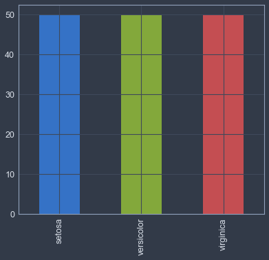
iris_data.species.value_counts().plot.bar()
<matplotlib.axes._subplots.AxesSubplot at 0x115a50978>
# x_name = 'sepal_width'; y_name = 'sepal_length'
# for species in pd.unique(iris_data.species):
#     x = iris_data[iris_data.species==species][x_name]
#     y = iris_data[iris_data.species==species][y_name]
#     plt.scatter(x,y, label=species)
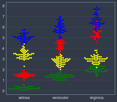
# plt.xlabel(x_name); plt.ylabel(y_name); plt.legend()sns.swarmplot(x="species", y='petal_length', color='red', data=iris_data)
sns.swarmplot(x="species", y="petal_width", color='green', data=iris_data)
sns.swarmplot(x="species", y="sepal_length", color='blue', data=iris_data)
sns.swarmplot(x="species", y="sepal_width", color='yellow', data=iris_data)
plt.xlabel(''); plt.ylabel('')Text(0,0.5,'')
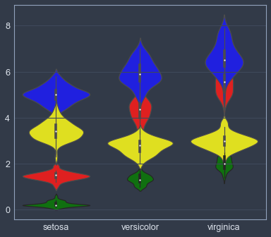
sns.violinplot(x="species", y='petal_length', color='red', data=iris_data)
sns.violinplot(x="species", y="petal_width", color='green', data=iris_data)
sns.violinplot(x="species", y="sepal_length", color='blue', data=iris_data)
sns.violinplot(x="species", y="sepal_width", color='yellow', data=iris_data)
plt.xlabel(''); plt.ylabel('')
Text(0,0.5,'')
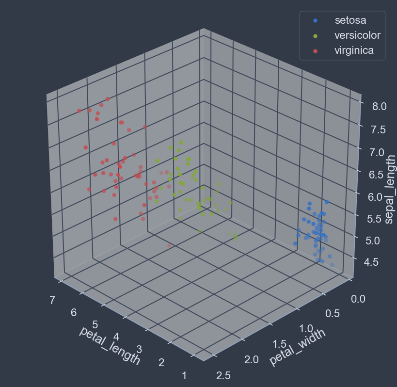
fig= plt.figure(figsize=(8,8), dpi=128); ax = fig.add_subplot(111, projection='3d')
x_name = 'petal_length'; y_name = 'petal_width'; z_name='sepal_length'
for species in pd.unique(iris_data.species):
    x = iris_data[iris_data.species==species][x_name]
    y = iris_data[iris_data.species==species][y_name]
    z = iris_data[iris_data.species==species][z_name]
    ax.scatter(x,y,z,label=species)
ax.view_init(30, 135)
ax.set_xlabel(x_name); ax.set_ylabel(y_name); ax.set_zlabel(z_name)
plt.legend()
plt.show()- The class 'setosa' is linearly well separated.
- The classes 'versicolor' and 'virginica' are likely not linearly separable.
- Classes seem to have good boundaries overall.
- Data forms some well defined clusters.
- Classes are mostly easily distinguishable by looking at cluster membership.
Judging by our exploratory analysis, not all classes can be completely separated via a hyperplane. However, the classes do seem to have well defined boundaries and are generally easily distinguishable. Therefore, some form of non-linear classification approach will likely yield better results: commonly by space partitioning via curved hyper-surface class boundaries.
Both SVMs (non-linear, via a feature space transform) and k-NN can be suitable for the task. However, due to the shape of the data, using an SVM will require an extensive hyper-parameter search as well as kernel comparison against various metrics, with no clear foreseeable benefits. Meanwhile, the data distribution looks well suited for a kNN to be quickly and easily trained without much tunning or computation.
By way of the above rationale, we'll choose to utilize the kNN algorithm.
# separate data into features and labels
X = iris_data.drop(columns='species')
y = iris_data.species
print('features: ', X.shape); print('labels: ', y.shape)
features: (150, 4)
labels: (150,)
# training validation split
X_train, X_test, y_train, y_test = train_test_split(X, y, test_size=0.1)
print('train split: ', X_train.shape, y_train.shape)
print('test split: ', X_test.shape, y_test.shape)
train split: (135, 4) (135,)
test split: (15, 4) (15,)
# randomization
X_train, y_train = shuffle(X_train, y_train)
# normalization
sc = StandardScaler()
sc.fit(X_train)
X_train_norm = sc.transform(X_train)
X_test_norm = sc.transform(X_test)# choose k-nearest-neighbors param
k = int(round(np.sqrt(X_train.shape[0])))
k12
# train classifier
knn = KNeighborsClassifier(n_neighbors=k, metric='euclidean')
knn.fit(X_train_norm, y_train)
KNeighborsClassifier(algorithm='auto', leaf_size=30, metric='euclidean',
metric_params=None, n_jobs=1, n_neighbors=12, p=2,
weights='uniform')
TODO: ROC, AUC, metrics, k values, visualize boundaries, SVM comparison, plot all 6 scatters, make 3d code more compact
# score classifier
print('Train Accuracy: {:.2f}'.format(knn.score(X_train_norm, y_train)))
print('Test Accuracy: {:.2f}'.format(knn.score(X_test_norm, y_test)))
Train Accuracy: 0.96
Test Accuracy: 1.00
link to MNIST dataset source website
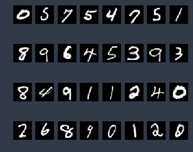
The dataset consists of 60,000 labeled samples. Each sample is a grayscale 28x28 pixel PNG image. Each image is labeled as a single digit from the range [0,9].
Note: this is not the original dataset in neither shape, form, format. We've done some pre-processing to it (outside scope of this notebook) for convenience.
# MNIST image directory and imag file extension
IMG_DIR = './mnist-images/'; IMG_FILE_EXTENSION ='.png'
# load file paths sorted by numerical value of file name, excluding the extension suffix
fpaths = sorted(os.listdir(IMG_DIR), key=lambda x: int(x[:-len(IMG_FILE_EXTENSION)]))
# load images
X = np.array([cv2.imread(IMG_DIR+fp, cv2.IMREAD_GRAYSCALE) for fp in fpaths],dtype=np.uint8)
# load labels
y = np.loadtxt('mnist_labels.txt',dtype=np.uint8)
# count and shape
print('X: ', X.shape,'\ny: ', y.shape)X: (60000, 28, 28)
y: (60000,)
# unique classes
np.unique(y)
array([0, 1, 2, 3, 4, 5, 6, 7, 8, 9], dtype=uint8)
# showcase a few samples
for ax in plt.subplots(4,8)[1].ravel():
    rnd = np.random.randint(0,y.shape[0])
    ax.set_axis_off()
    ax.imshow(X[rnd],cmap='gray')
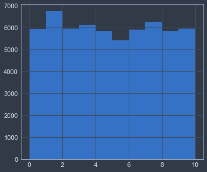
# plot class sample counts
plt.hist(y, bins=range(11))(array([ 5923., 6742., 5958., 6131., 5842., 5421., 5918., 6265.,
5851., 5949.]),
array([ 0, 1, 2, 3, 4, 5, 6, 7, 8, 9, 10]),
<a list of 10 Patch objects>)
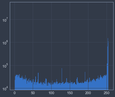
# plot logarithmic grayscale color histogram
hist = plt.hist(X.flatten(), bins=range(256), log=True)
# compute and show average pixel values for each digit class
avgs = np.hstack([np.mean(X[y==i], axis=0) for i in range(10)])
plt.matshow(avgs,cmap='gray'); plt.axis('off');# compute and show median pixel values for each digit class
medians = np.hstack([np.median(X[y==i], axis=0) for i in range(10)])
plt.matshow(medians,cmap='gray'); plt.axis('off');# compute and show standard diviation of pixel values for each digit class
stds = np.hstack([np.std(X[y==i], axis=0) for i in range(10)])
plt.matshow(stds,cmap='gray'); plt.axis('off');# training validation split
X_train, X_test, y_train, y_test = train_test_split(X, y, test_size=0.3)
print('train split: ', X_train.shape, y_train.shape)
print('test split: ', X_test.shape, y_test.shape)train split: (42000, 28, 28) (42000,)
test split: (18000, 28, 28) (18000,)
# randomization
X_train, y_train = shuffle(X_train, y_train)
# threshold and binarize the images
X_train = np.where(X_train>127,1,0).astype(np.bool)
X_test = np.where(X_test>127,1,0).astype(np.bool)
plt.matshow(np.hstack(X_train[:10]*255),cmap='gray'); plt.axis('off');# flatten images to match classifier,preprocessors,etc expected input shapes
X_train = X_train.reshape(len(X_train), -1)
X_test = X_test.reshape(len(X_test), -1)
print('X_train:', X_train.shape,' X_test:', X_test.shape)X_train: (42000, 784) X_test: (18000, 784)
# standarize and perform PCA dimensionality reduction
pca = PCA(0.65, whiten=True)
X_train = pca.fit_transform(X_train)
X_test = pca.transform(X_test)
print('X_train:', X_train.shape,' X_test:', X_test.shape)
X_train: (42000, 34) X_test: (18000, 34)
# plot inverse PCA result
plt.matshow(np.hstack(pca.inverse_transform(X_train[:10]).reshape(-1,28,28)),cmap='gray'); plt.axis('off');
# tsne = TSNE(n_components=2, n_iter=250)
# tsne.fit(X_train)MNIST is a larger dataset with many more dimensions and training samples (~5m even in binary form). Although it's still not large enough to make kNN classification computationaly unfeasible, it's probably a better direction to utilize something like a linear or polynomial SVM since it's likely to be a much more efficient classifier.
# setup SVM hyperparam search
hyperparams = {'kernel':['linear', 'poly','rbf'],'C':expon(scale=10), 'gamma':expon(scale=0.1), 'degree':randint(3,7)}
rand_search = RandomizedSearchCV(SVC( ), hyperparams, n_jobs=-1)%%capture
rand_search.fit(X_train,y_train)# rand_search.best_params_
# rand_search.best_estimator_
# rand_search.score(X_test, y_test)
y_pred = rand_search.predict(X_test)
print(classification_report(y_test,y_pred)) precision recall f1-score support
0 0.99 0.99 0.99 1771
1 0.99 0.99 0.99 1970
2 0.97 0.97 0.97 1812
3 0.96 0.97 0.97 1807
4 0.96 0.98 0.97 1749
5 0.97 0.96 0.96 1589
6 0.98 0.99 0.98 1804
7 0.97 0.97 0.97 1874
8 0.97 0.96 0.97 1786
9 0.97 0.96 0.97 1838
avg / total 0.97 0.97 0.97 18000
