This repository contains contents for teaching SoS crews how to set up and interact with the open source, lightweight, and efficient geographic information system (GIS) QGIS.
A Geographic Information System (GIS) is a system that is used for displaying, analyzing, and in part distributing data which have geographic attributes. As of the last few decades, GIS are nearly synonymous with computers, although they predate them. Several different GIS softwares exist. The most popular are generally: R, Python, GrassGIS, SagaGIS, QGIS, and ArcGIS - which is being superseded by ArcPro. The 'Arc' line of products are produced by the company ESRI, and are very popular in multiple tiers of government in the United States (e.g. city, county, state, and federal). The other Geographic Information Systems are very popular in academic settings (Universities, or the Research Divisions of Government Agencies like the USGS), and worldwide. Most of these earlier systems are all Open-source, which means individuals and organization are able to contribute code to improve their performance for certain applications. Most of these other GIS software compose a ecosystem, where some rely on others.
QGIS is arguably the most common GIS in the open source ecosystem with a Graphical User Interface. Many appreciate that it is 'light', i.e. it does not take up enormous computer resources which allows it to load very fast and be responsive to users panning and toggling around the map. We will use QGIS as a supplement to the ESRI Geoplatform product. This is simply due to the fact that we have generated a ton of data which I do not have access to add back to the BLM servers! Such is government.
Normally, I would not ask you to install GIS software on your computer; but due to being so 'light' QGIS is the exception. QGIS can be downloaded from here, for all major operating systems: Windows, Mac, and several flavors of Linux.
Windows users are very unlikely to need the OSGeo4W installer; although it is a small efficient piece of software which does not take up much room. It might be safer to download than be sorry if you want to keep using this in the not so near future!
Mac "macOS High Sierra (10.13) or newer is required. QGIS is not yet notarized as required by macOS Catalina (10.15) security rules. On first launch, please control-click on the icon and choose Open from the context menu, after which a confirmation dialog is shown and you need to click the Open button."
There is a common problem on Macintosh that the security ticket from QGIS is not recognized. This should have been fixed a long time ago, but this post details how to bypass security to allow usage of QGIS. To do this: Apple Menu > System Settings, then click Privacy & Security . In the lower half of this window you should see a message similar to: "QGIS3.10 can't be opened because Apple cannot check it for malware" click Open anyways and then, if another window pops up open. QGIS shoult now be on your approved list of software and you now be able to open it as needed!
Linux please refer to this additional page on installation
Great that is about it! It is a quick install! Once downloaded navigate to the program, and if necessary feel free to pin it to your start bar or something so you don't forget about it! You can now delete the 'installer' from your downloads - the program is installed elsewhere one your system and the installer is no longer required.
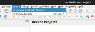
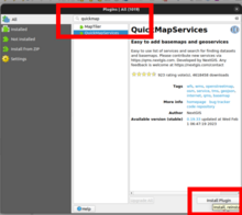
Part of why QGIS is so light it that it does not come with many interfaces to the other open-source software which some folks may use. You download these using Plugins - Plugins are like apps. We will install two Plugins. Open QGIS, if it is not already, and navigate to the Plugins tab on the top bar and Plugins >> Manage and Install Plugins. From this pop-up screen use the Search bar at top to search for QuickMapServices. We will use this Plugin to display base maps. Now let's add one more Plugin, using the Search bar search for Load Them All. We will use this service to import many files quickly.
Part of why QGIS is so light it that it does not come with many interfaces to the other open-source software which some folks may use. You download these using Plugins. We will install two Plugins. Open QGIS, if it is not already, and navigate to the Plugins tab on the top bar and Plugins >> Manage and Install Plugins. From this pop-up screen use the Search bar at top to search for QuickMapServices. We will use this Plugin to display base maps. Now let's add one more Plugin, using the Search bar search for Load Them All. We will use this service to import many files quickly. We will grab another Plugin which we can use to order our species by alphabetical names later. Layer Group and Sort
That's it! We now have an operational GIS on our hands!
You all should have been sent a folder of data tailored for your region. The data will be in a zip file; this is a formatting for compressing data which makes it easier to send. Please download this file. Once downloaded (or if you have the change to before), please drag this to your project specific folder for Seeds of Success this year.
A good place to put this folder, if you do not already have it, is in your Documents. A suitable path, and name for this folder should be "C:/UserName/Documents/2024SOS_Planning". Notice that we are not keeping these data on OneDrive, we want them copied onto your physical drive. This will allow you to review these data without internet connection.
Drag and drop this folder from your downloads into this location, and unzip the folder. On most software systems you can right click the file, and select an option like decompress. This folder contains a ton of supplemental project data. Most importantly it contains Species Distribution Models (SDMs), we generated species distribution models for most of your species. Species that we skipped were generally super abundant and you shouldn't have too much trouble finding them. If you would like to learn more about SDM's please visit this lecture I recently gave. This folder also contains occurrence data for the species, a subset of the records here are identical to those on the tablet, but we have several times more! We used this large data set of occurrences to create our Species Distribution Models.
The only other data sets we have which are not present on the tablet are some data on Drought, Invasives annual grasses. If you are interested in learning more about Ecological Drought check out this section of a big ol' government report here, and some more good info on invasive species from the same report can be found here. Cool! So while these data are very similar to what is on the tablet, we have a few more tricks up our sleeves as you will see.
Now we are also going to download some data that contains pre-specified aesthetics for our project. I have been able to load and pre-style all but two components of these projects.
We will need to manually drag in both the raw species occurrence data, as well as the SDM's which have been clipped to hydrologic basins.
Many GIS operate on the sense of a project a big related set of objects for each thing you are working on. We have already created a project for you 'HitchPlanner.qgz', and added many data sets which you will use while hitch planning.
.
├── Admin
├── Disturb
├── HitchPlanner.qgz
├── qml_styles
├── Roads
├── Species
└── STZ
If you are unfamiliar with the root, it is the base of something! So if we look in the geodata folder, and think of it as the soil, we have 'Admin', 'Disturb', 'Drought', 'Roads', 'Species' and 'STZ' all rooted in it!
the root of a specific projects directory is:

Let's launch our 'HitchPlanner' project by double clicking on it.
Note that you will need to manually drag the focal area to where your crew is actually operating. It is defaulting to the field office which I set up first to 'style' the elements.
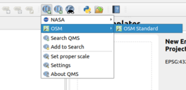
We are now ready to import data to our QGIS project, it looks a little sad without any content doesn't it? First let's add in a base-map so that we are oriented. We will use the QuickMapServices Plugin which we just installed. This Plugin is generally located on the right end of your toolbar. It looks like a globe with binoculars.
Once you have located it, we will use it to import the standard base-map which it ships with, OSM >> OSM Standard. This imports a freely available base map tile service. Cool!
Now we will import our two big sets of data, our Species Distribution Models, and the occurrence data we used to create them. These are most complex imports, so we will do them before we have a chance to mess up the project and need to revert back! We are now ready to import data to our QGIS project.
Now we will import our two big sets of data, our Species Distribution Models, and the occurrence data we used to create them.
find-directory-vector.mp4
We will utilize our other plugin Load them all, load them all looks like a folder with a green arrow coming down from it, like the folder is being opened. So click on that! Now make sure that the leftmost option, Vector, is toggled. Vector data are what sometimes are called 'shapefiles', shapefiles are a specific type of vector data, but not all vector data are shapefiles!!! If you are unfamiliar with geographic data formats, check out a lecture on the topic here. We will now navigate to the to the folder containing your geodata 'Geodata/Species/Occurrences', and select the file format ESRI Shapefile (*.shp). Now at the very bottom right of this window select 'Load Data'.
Ok now the occurrence data are imported! We are going to turn these into a Group, a set of data which we can manage simultaneously. To create a Group right click on the top-most record scroll down to the very last record, and right click again while holding shift. With any luck every record will now be selected! Now on drag these records into the 'Occurrences' group which is nested within the Species group.
Group-Selected.mp4
We will style these data now quickly. Because well, they are uninformative, and data which are uninformative are not worth much. We will load some pre-loading styles I came up with using Colorbrewer, hopefully they look okay. Right click on the top-most species occurrence record and select 'Properties' and then Style >> Load Style, now navigate to the qml_styles directory, and select the Occurrences.qml file. Now Apply and OK this selection.
For the 2024 data, 'Occurrences' is still the name for the occurrence point data, and 'SDM-Pred' is the name for the species distribution data which you have been sent.
Load_style-single.mp4
You might not even be able to see what we did there... Let's turn of all of the records in our Occurrence group really quick. Right click on the group, and select Uncheck and all it's children, now just check the little cell next to the record you added the stylings to, maybe Achnatherum lemmonii, OK see what we did? If not you might need to Right Click >> Zoom to layer; now you should be focused on these records. Keep in mind for you field offices there could only be 1 record!
Now, let's apply this styling to every species in our Occurrence group. Click on the name of the top-most record and Style >> Copy Style >> Symbology, and now right click >> Paste style. If all goes to plan, each species will have the same symbology!
But wait... why? Why should each species be the same color! This makes no sense!!! So, the way we came up with this stuff is using a lot of code and approaches from a technique called 'Data Science', I'm sure you have heard these term, there is a lot of hype around it. One of the fundamental rules of data science is don't get overwhelmed by data. So I seriously, suggest, that you look through each species one at a time! Yep... more on this later. You will also notice that their are several sets of symbology within this layer; the older a record the lighter the color; you will also notice you can deselect old records? Why, because many of those old populations may no longer exist; we want to use current data.
Now if that all went to plan, let's save our project! Now we can add in the SDMs
A very similar process is used to the bulk importing of Species Distribution Models as for the raw occurrence data.
We will need to select the second tab on the Load them all plugin pop-up window. We will the redirect the path to the SDM. Now you can load the data again. They should also be grouped and have their styles added to them in the same way as the occurrence data.
Note that we dramatically changed how we distribute SDM's for the 2024 year, we nor distribute them as vector data? Can you tell what we clipped these data to? Hydrologic basins.
If you recall all that a species distribution model tells us is the probability of suitable habitat in each cell. They do not incorporate information regarding the possibilities or probabilies of dispersal from a known site to an unknown site. In the above dataset we have done two steps to try and make models more representative of a likelihood of colonized habitat. First we have masked areas with less than 80% probability of suitability, in other words we want their to be a very high likelihood that the habitat is actually suitable. Second we have clipped these suitable areas to hydrologic basins. These areas are expected to have high movement of propagules within them, but depending on the topographic relief, and the relative orientation of them, less movement between them. We have assigned a rank to each patch of suitable habitat within a basin, based on it's 'distance' to a patch which we know is populated.
- '1' indicates that a patch is truly occupied (at least in recent history) in at least part of it's extent.
- '2' indicates that a patch neighbors two or more occupied patches, e.g. is a basin just over a ridge - this ridge may be virtually flat and unlikely to restrict flow of seeds, or very steep and likely to restrict flow of seeds.
- '3' indicates a patch borders a single occupied patch.
- '4' indicates that a patch has at least three neighbors which are adjacent to a '1'.
- '5' indicates that a patch has two or less neighbors which are adjacent to a '1', or that three or more '1's exists within 5 kilometers of it.
- '6' indicates that a patch has four or more neighbors which are adjacent to a '2', or that a '1' exists within 5 kilometers of it.
- '7' indicates that a patch has three or fewer neighbors which are adjacent to a '2'.
I expect most 1 and 2's wills be occupied, and that just about half the '3' and '4' will be occupied. 5's and up seem like losing gambles to me.
If you have few of these polygons for species in your area, let me know and I will send you the 'raw' SDM output. Some areas suffer from a lack of recent field work, and this approach is not optimal for them.
Now remember that QGIS draws layer in ascending order based on the box in the left hand of the screen. Please move the Occurrence type points above the clipped SDM polygons. This will allow you to see both the points and polygons at once.
If you want to be able to see through the polygons you can change the opacity. Click on one of the species in your stack, under the 'Symbology' tab (left side) in the window, click the pink bar in 'Symbol'. Drag the Opacity bar down to 70% or so. Click 'OK', and then 'OK' to exit the window and the selected layer should be updated. Now with this layer selected 'Styles' -> 'Copy Style' -> 'All Style Categories', and you can then paste it to the top most record in this group (described above), and all layers should take on this style.
If you want to make the occurrence points larger we can do that too. Select the layer for a single species, once it is highlighted in blue, right click and select 'Properties', now you should be in a window with 'Symbology' toggled to the left. Click the arrow next to 'Symbol' and 'Configure Symbol'. Now into the Size field type in '15' or so, hit 'OK' and 'OK' again. If this size is large enough, copy it to the other layers within this group as described above.
Some of the layers are kind of redundant and some will require only cursory glances at. For example, the 'Drought' layers are oftentimes pretty similar, and easy to interpret. Anywhere that is not in negative values is great to collect from! And theoretically the bluer, the area the more seeds. But don't worry too much about trying to maximize this.
Drought-toggle.mp4
Speaking of drought, because the moisture has been pretty good this season, it is a good year to collect from some of the dried Seed Transfer zones, I have added them in. If we toggle this on and off, you will notice there are some small patches of land which are not colored, these zones are NO GO's! They are too small and it is not desirable to collect seed from them. Depending on where you are working, BLM may not really have any land in them anways!
STZ-BLM-overlap.mp4
We can readily look at the relationships of Fire and Invasive annual grasses here. Note that historic fires beg fires to re-occurr, this is common, and that these areas often have the highest amount of invasive species! Hmmm....! You'll hear alot about this this year! Essentially these annual invasives have totally altered the fire-cycle and are caught in a positive (for them...) feedback loop!
Fire-Invasive-Species.mp4
Finally, we can show how to focus on a single species to look at some prospective areas for scouting. Here we will add the occurrence records, by time period, and then add on the Species Distribution Models. As you can see occurrence records explode since the millenium, this is largely due to the implmentation of the AIM program around 2010. The SDM has been categorized into 5 classes, the first - which you cannot see, is highly unsuitable habitat. The next four levels go from 1-4, and indicate increasingly suitable habitat. Classes 3 and 4 are very suitable and ideal, respectively.
Adding_SDM_to_occ.mp4
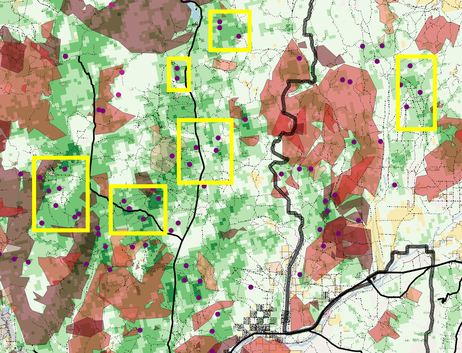
Now we can use some relevant layers to look for some areas which like promising scouting locations. Most all of these areas look pretty good! Although the lower left most looks pretty close to private, and deserves closer investigation. The furthest right most population looks pretty far off the beaten path, and the road conditions to it should be investigated; if things don't pan out at the populations near the major roads it is worth asking BLM staff about conditions out that way.
Identify-prospective_populations.mp4
Here I have drawn some simple yellow boxes around a few of these candidate areas.
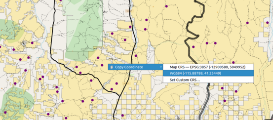
There are many different ways to get to these. Which one you choose is pretty personal. An old-timer like me will grab the coordinates, mark them in a physical road atlas, and navigate to them using that, using BLM 1:100 topos as required. But, your tablets provide excellent alternatives!!! For example you can drop pins to these in there, or even select the AIM plot records!!!
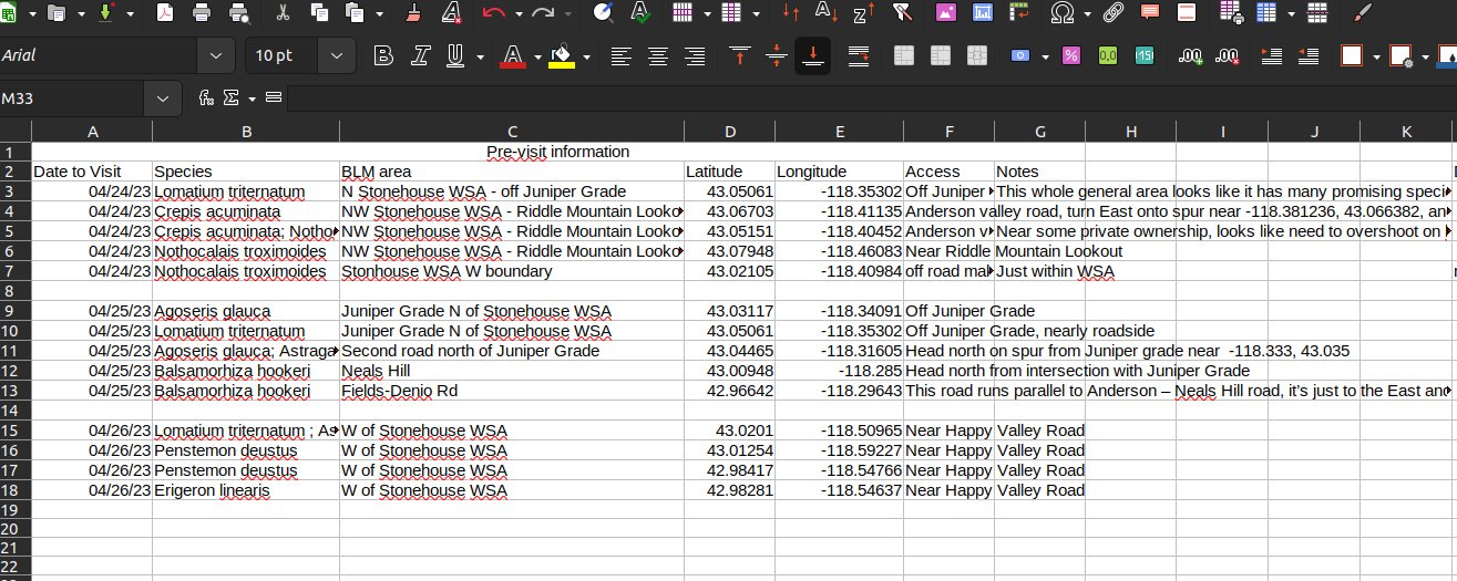
Anyways, hopefully you have QGIS set up now, and you can start finding scouting populations one species at a time! Whether you record locations in road atlases, tablets, or whatever else, we encourage you to put them on a spreadsheet. Then you have a record of what looks promising, and we expect you to record the fate of each of these scouting events to the tablet! After a few scouting hitches, you will then be able to switch exclusively to geo-platform for your collection revisits!!
The above example is a good way to start focusing on species and to keep track of your upcoming hitch (or maybe one far off in the distance depending on when the species flowers). You can more or less group points onto the same day as each other for scouting.
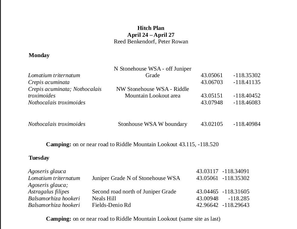
A tracking spreadsheet like this will also allow you to create a hitch plan very quickly. We want you to make hitch plans so that we have an idea of where you are in the field! While these can be pretty complex for some jobs, our requirements are pretty minimal; and we want them to be useful to you and not entirely an obligation.
Also add a simple screenshot of the general area(s) you plan on going.
the above image is more than enough detail, and if you look closely you will see it contains some of the named roads. (you can turn road names on in QGIS via right clicking the 'roads' data set, and then show labels; show labels is about the fifth item down on the pop up; but bear in mind, most BLM roads are unnamed, so you may need to zoom out to see if it's working!).
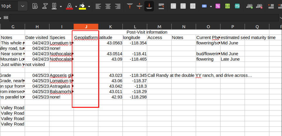
Once you return from your hitch you can add some more tracking info to the sheet. I think the easiest solution is to mostly just link the population back to the scouted point, and copy out the pieces of info which you think you will need to remember to go back to the plot using the tablet!

