
The goals / steps of this project are the following:
- Use the simulator to collect data of good driving behavior
- Build, a convolution neural network in Keras that predicts steering angles from images
- Train and validate the model with a training and validation set
- Test that the model successfully drives around track one without leaving the road
- Summarize the results with a written report
The project includes the following files:
model.py- containing the script to create the modeltrain.py- containing the script to train the modelvalid.py- containing the script to validate the modeldrive.py- for driving the car in autonomous modemodel.h5- containing a trained convolution neural networkregistry.py- containing helper class for handling driving logreader.py- banch of helper classes to iterate through data pointsrepository.py- helper class the provides git-like filesystem layout for huge directoriesgenerator.py- core routines for data generationpipeline.py- pipeline definition for training and validationcvutils.py- bunch of routines used in data augmentationREADME.md- project quick overview and summarizing the results
Model can be trained using following command
python train.py -t dataset/driving_log.csv model.h5Input:
- dataset/driving_log.csv - path to driving log
- model.h5 - path to model
Output:
- model.checkpoint - directory containing model snapshot for each epochs
- model.test.csv - fraction of original driving log which was not used in training process, could be used for validation
- model.history.p - pickled version of training history
Model performance could be measured by following command
python train.py -v dataset/model.test.csv model.h5Input:
- dataset/model.test.csv - validation data set
- model.h5 - model
Output:
- loss - will be printed on console
Using the UdaCity provided simulator [1] and my drive.py file, the car can be
driven autonomously around the track by executing
python drive.py model.h5 [output]The overall strategy for deriving a model architecture was to:
- Collect relevant training data
- Analyze collected data to better understand it
- Preprocess and normalize collected data
- Use appropriate data augmentation techniques
- Tune network parameters in order to achieve the best performance
- Validate model on the simulator
My first step was to use a convolution neural network model similar to the one described in [2]. I thought this model might be appropriate because the original work was focused on the similar task.
In order to gauge how well the model was working, I split my image and steering angle data into a training, validation, and test sets. See data analyze section for details.
At the end of the process, the vehicle is able to drive autonomously around the track without leaving the road.
Training data was chosen to keep the vehicle driving on the road. I used a combination of center lane driving in forward and backward direction, recovering from the left and right sides of the road.
To capture good driving behavior, I first recorded three laps on track one (lake) trying to keep center lane driving. Here is an example image of center lane driving:

I then recorded the vehicle recovering from the right side and left sides of the road back to center so that the vehicle would learn how to fix position on a road. This animation shows what a recovery looks like starting from left side:

Next I recorded three laps on track one of center lane driving in opposite direction.
Then I repeated this process on track two (jungle) and track three (castle, found in previous version of simulator) in order to get more data points.
After the collection process, I had 53688 data points. The data points were divided to training, validation and test sets (randomly shuffled). The actual numbers are
| Name | % | # of points |
|---|---|---|
| Training set | 70% | 37581 |
| Validation set | 12% | 6442 |
| Test set | 18% | 9665 |
Raw data distribution presented on figure below. Note logarithmic scale.

'Straight driving' pattern was over represented in the data, which may lead to biased network which unable to steer. In order to prevent high 'go straight' bias I filtered out 80% (the parameter chosen experimentally ) of data points with 0 steering angle. The distribution changed to the following (still over represented, but better).

Bellow I described augmentation techniques used in the project.
In order to obtain more data points in a safe way images were flipped around y-axis, steering angle changed sign. The technique makes sense since it produces valid (which may be captured by camera) image and appropriate steering angle. This technique might lead to model overfitting since representation of some features doubled.

The simulator provides two additional (left and right) images for each data point. This images may be used in training process. The biggest problem is to find appropriate steering angle correction. Also one have to keep in mind the correction angle will be over represented in the data (since 'go straight') is over represented. After several experiments with static and random correction angles, I choose correction angle to be normally distributed with mu=0.1, sigma=0.03. Randomization in my opinion should reduce chance of overfitting.
Another possible augmentation technique - random brightness and/or contrast adjustment. Using this technique allows model to learn how to deal with different light conditions (sun sets, mid-days, shadows). Randomization reduces chance of overfitting.
I used brightness adjustment with uniform distributed in range [-20, 20].

Rotation could be used to produce more data. For example slightly rotated images could help the network to learn how to drive in hilly environment (ie. jungle track).
The thing a believe helps a lot with fighting against overfitting - steering angle randomization. The nature is continuous. In most cases small change of value will not change final behavior, but will allow to smooth data distribution. I my experiments I used normally distributed randomization with mu=originalAngle and sigma=0.003
Training data grooming pipeline
- Angle adjustment for images from left and right cameras
- Flipping images
- Random brightness adjustment
- Generating N (2 in my case) additional images using rotation
- Angle randomization
Sample of all images generated from one data point (N=1):

Data distribution after pipeline:

Each image pass the following preprocessing steps before feeding into the network (some steps implemented as lambda layers)
All images converted to YUV colorspace as proposed in [2].
Since top of each images shows sky and landscape (which is not much useful for the task) and bottom shows parts of the car. Obvious decision is to crop the image in order to reduce size (less to data to process) and focus network on useful details.

Each channel of an image normalized in order to have value in range [-1, 1].
The final model architecture (model.py) consisted of a convolution
neural network with the following layers and layer sizes
| Layer | Input | Output | Kernel | Filters | Stride | Activation |
|---|---|---|---|---|---|---|
| Cropping | (160, 320, 3) | (80, 320, 3) | ||||
| Lambda | (80, 320, 3) | (80, 320, 3) | ||||
| Convolution | (80, 320, 3) | (38, 158, 24) | (5, 5) | 24 | (2, 2) | ReLU |
| Convolution | (38, 158, 24) | (17, 77, 36) | (5, 5) | 36 | (2, 2) | ReLU |
| Convolution | (17, 77, 36) | (7, 37, 48) | (5, 5) | 48 | (2, 2) | ReLU |
| Convolution | (7, 37, 48) | (5, 35, 64) | (3, 3) | 64 | (1, 1) | ReLU |
| Convolution | (5, 35, 64) | (3, 33, 64) | (3, 3) | 64 | (1, 1) | ReLU |
| MaxPooling | (3, 33, 64) | (1, 31, 64) | (3, 3) | (1, 1) | ||
| Flatten | (1, 31, 64) | 1984 | ||||
| Dense | 1984 | 100 | ReLU | |||
| Dense | 100 | 50 | ReLU | |||
| Dense | 50 | 10 | ReLU | |||
| Dense | 10 | 1 | Linear |

All layers except the output use ReLU activation to introduce nonlinearity. The model includes ReLU layers to introduce nonlinearity. Model uses Keras cropping and lambda layers in order to prepare (crop and normalize) input data.
There is no dropout layer in the model, see next section for thoughts about overfitting/underfitting.
I used this training data for training the model.
- Loss function - mean squared error - reasonable choice for regression model
- Optimizer - Adam - adaptive learning rate simplifies learning and reduces number of hyper parameters
- Batch size - 768 - when using AWS/Azure high performance servers for training there is no limitation on RAM, and batch size could be chosen as big as graphics card memory size allows, since transferring data between RAM and graphics card memory could become a bottleneck.
- Number of epochs - 30
Learning curve for training:

Key observations and potential explanations:
- Model seems to be under trained - loss on training set keep going down. On other hand loss on validation set doesn't change a lot. This could be a sign of overfitting, so stopping at reasonable number of epochs good enough.
- Even without dropout or other regularization techniques model doesn't look
overfitted. In my opinion reasons are
- Relatively small number of parameters
- Massive randomization of input and measurement
- Huge disproportion of 'go straight' is good in fact. The network seems new examples from this category each epoch
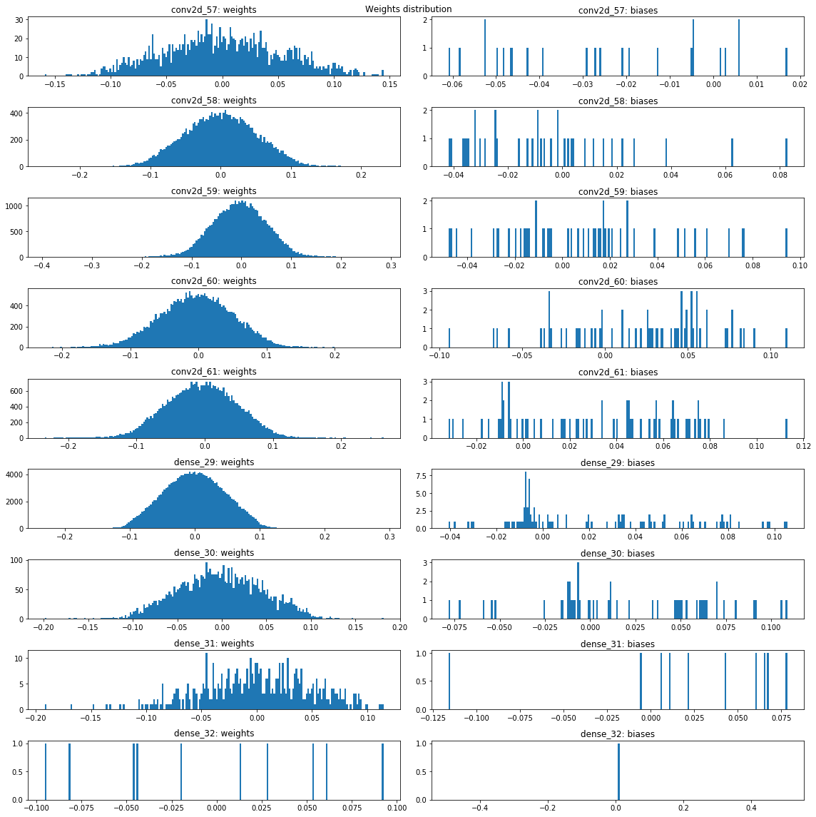
- Figure below shows weights and biases distribution, which looks sane.
Weights tend to be normally distributed around 0 within reasonable range.
This make me think L2 weights regularization will not help much.

The validation set helped determine if the model was over or under fitting. Finally test data helped to determine real model performance.
The model was tested by running it through the simulator and ensuring that the vehicle could stay on the track.
- Generate train data batches with GPU, currently CPU used
- Generate train data batches using multiprocessing, single core used currently
| Name | Link |
|---|---|
| UdaCity training data | https://mega.nz/#!V9tASADT!TV_YZUTJi9pNRUG1j7Raev0oK3KbUgszAJkKKxOiXL8 |
| Track 01 forward direction | https://mega.nz/#!Z0dhDITD!XWJcWTTS9-67PndO2cgstjxdJcoaTEGY9yohW3geD8Y |
| Track 01 backward direction | https://mega.nz/#!RxNwkbza!BzeH7kLL133YO2CbUQUMMDCdsGe3q_Z_N7FoaAOBcDU |
| Track 01 random samples | https://mega.nz/#!18ciRCzR!_6Pu0JHbsEi2gn8PmHTJPEK8EsPsX2jorCoGY3qExIU |
| Track 02 forward direction | https://mega.nz/#!xs9H3Yqa!82WpBN9cZIYMKaV9_hFgi4pqnP2Xiy6jlWJN-dKvssE |
| Track 02 backward direction | https://mega.nz/#!048UlLgI!CBciscwULl_zYg4H3btm95XU0WJKxGFgGvJ3SrE5JbM |
| Track 02 random samples | https://mega.nz/#!NhkhUIqL!S-TvoKj_y4C8Gmt_FsxRVN15XUPPcEbfQ_emSvJVLYQ |
| Track 03 | https://mega.nz/#!VgMGXZSL!iT-DiEYqiVcZjZ8F-34C8b01bhT3C6Av4i8_TUpOY6s |
| Track | Car View | Simulator View |
|---|---|---|
| track01 - lake | https://vimeo.com/234067418 | https://vimeo.com/234067436 |
| track02 - jungle | https://vimeo.com/234067565 | https://vimeo.com/234067584 |
| track03 - mountains | https://vimeo.com/234067698 | https://vimeo.com/234067714 |
- Udacity's Self-Driving Car Simulator https://github.com/udacity/self-driving-car-sim
- Bojarski, M., Del Testa, D., Dworakowski, D., Firner, B., Flepp, B., Goyal, P., Jackel, L. D., Monfort, M., Muller, U., Zhang, J., et al. (2016). End to end learning for self-driving cars. arXiv preprint arXiv:1604.07316.