ML Algorithms from scratch Python (Learning Repository)

This repository contains the implementations of popular Machine Learning Algorithms in python without using in-built libraries.

Datasets Used

The algorithm terminated on its own after I ran some epochs for the linearly-separable dataset. The algorithm gets converged when the training error (empirical risk minimization) comes out to be 0. This algorithm terminated because perceptron algorithm handles only linearly separable datasets.
The heuristic that I took for the termination of the algorithm is by comparing the training error of four consecutive epochs. When the error remains constant then I terminate it.
For the breast_cancer_dataset, the algorithm did not converge i.e. it did not terminate as intended.
As per the experiments, breast_cancer_dataset is not linearly separable so this is the reason why the algorithm did not terminate.
Training Error did not converge to 0, so we can infer that the algorithm for this dataset will not converge since breast_cancer_data is not linearly separable.
The runtime of linearly-separable is less compared to breast_cancer_data since breast_cancer_data is not linearly separable.

Mode: erm / kfold (For cross validation, number of folds = 10 by default) / plot (for plotting graph b/w ERM and Validation error vs Rounds)
Rounds: Integer variable

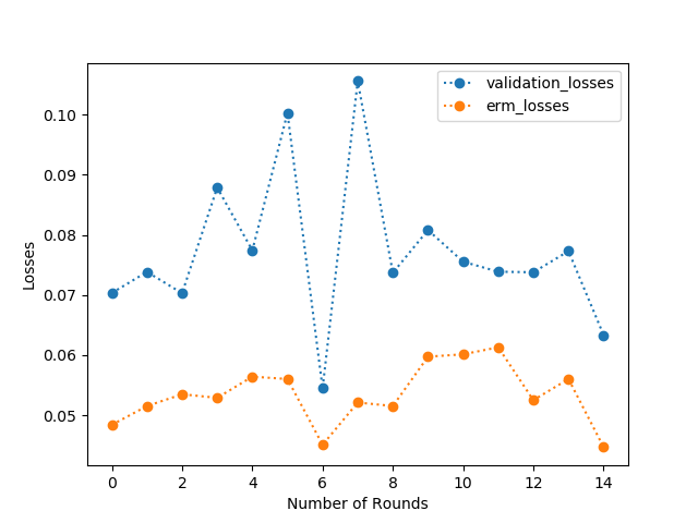
As you can see that the plot (Figure 1) below clearly depicts that the validation loss is at all times more than the empirical loss.
This behaviour shows that the training folds yield less loss compared to the test folds. According to the figure, I would recommend 15-20 rounds(epochs) to clearly show the difference between the empirical and validation loss.

dataset: Breast_cancer_data.csv
distance: default='euclidean' otherwise it takes values as 'cosine', 'manhattan'

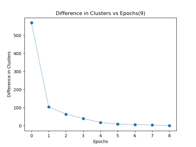
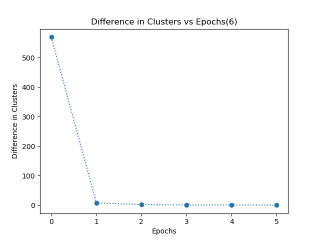
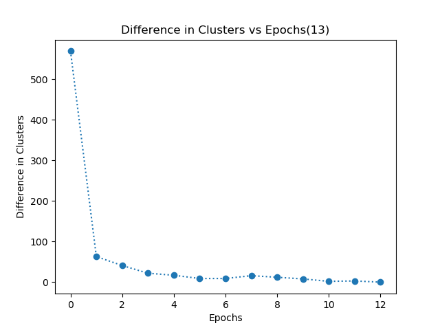
My k-means algorithm converges when each data point in the dataset has the same cluster allocation for consecutive 2 epochs. I have even plotted a graph of difference in clusters vs epochs. This graph shows the number of data points which have different clusters in two consecutive epochs.

Euclidean

Manhattan

Cosine

I observed that when k=2 i.e. when we have to divide the dataset into 2 clusters, each cluster can clearly divide the dataset into 2 clusters based on the diagnosis label. This is shown in the table below. I have calculated the percentage of data points having 0 as diagnosis in both the clusters and similarly, diagnosis of 1 in both the clusters.

Required arguments:

I have normalized the dataset to prevent biasing of features and I have split the dataset into 80% training and 20% testing.
Evaluation of dataset is done by predicting the label of each test instance.
Prediction of each instance is done by calculating the euclidean distance of each test instance with all the data points in training data.
Then sorting the distance in ascending order and extracting the labels of the first k data points.
The final label of test instance is the majority label of its k nearest neighbours that I extracted in the previous step.
This is how I evaluated all my testing instances.
Accuracy is calculated by comparing the predicted label and actual label of the respective testing instance.
Obtained an accuracy of around 89% - 93%.
To generalize the accuracy, I have done this for a number of epcochs, then calculated the average accuracy over epochs.

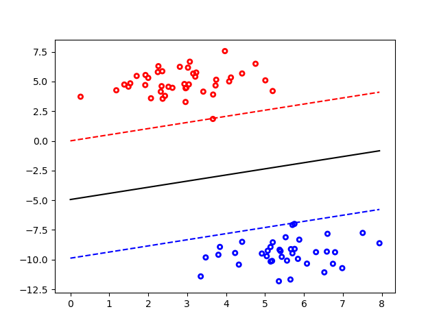
A Support Vector Machine (SVM) is a discriminative classifier formally defined by a separating hyperplane.
In other words, given labeled training data (supervised learning), the algorithm outputs an optimal hyperplane which categorizes new examples.
In two dimentional space this hyperplane is a line dividing a plane in two parts where in each class lay in either side.