sisl/RunwayPNPSolve.jl

PNPSolve Repository

This repository contains the libraries, experiments, and reports developed during the 2023 Summer internship by Romeo Valentin (romeov@stanford.edu or romeo.valentin.int@airbus-sv.com).

TLDR: The report can be found at ./report.pdf.

The libraries contain tools to solve the PNP problem using simulated runways and airplane positions and attitudes.

Library overview.

We provide three libraries:

• RunwayLib.jl deals with loading runway data from csv and spreadsheet files, settup up the coordinate systems, and computing the projections.
• LsqPnP.jl deals with solving the PnP problem, including pixel coordinates and hough-transform. We currently use the Levenberg-Marquardt method, but have also had good results with Trust-Region Newton Method. A short performance benchmark is discussed below.
• PNPSolve.jl acts as the glue, setting up all the experiments, plotting, interactive visualization, etc.

Performance.

We currently achieve about 350 pnp solves / s on a single core, and about 1000 pnp solves / s when multithreaded on an 2.7 GHz Quad-Core Intel Core i7 (>5 years old). See benchmarks/pnp_benchmark.jl for the experiment setup.

Report.

The report can be found at ./report.pdf.

Reproducing the experiments.

The experiments are managed by the PNPSolve.jl library itself. We try to set it up in a way that you can just run julia --project scripts/run_all_experiments.jl to regenerate all the plots.

Interactive simulator.

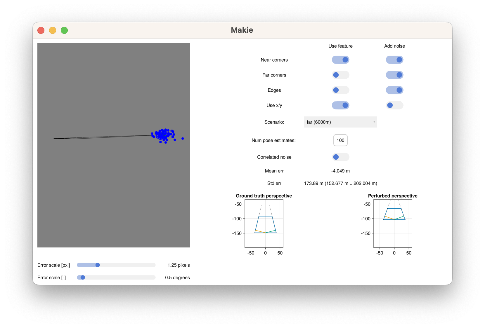
This library provides an interactive PNP Simulator based on Makie.jl that allows for dynamically changing the airplane setup, the magnitude of the noise, etc, and collecting statistics about the error distributions. The visualization is GPU accelerated and the computation is CPU parallelized, which leads to real-time performance.

There is some additional performance statistics implemented, but currently not part of the GUI. Will probably make a comeback.

Used libraries.

We use

• Geodesy.jl and CoordinateTransformations.jl to set up statically typed coordinate systems, implemented as typed statically sized vectors (basically tuples), and provide our own implementation of GeodesyXYZExt.jl that sets up a runway local reference frame and enables easy coordinate transformations.
• StaticArrays.jl and specifically FieldVector backs up all the array data types to provide autogenerated super fast code.
• LsqFit.jl to solve the least-squares reprojection error using a Levenberg-Marquardt method. We also tried Optim.jl and LeastSquaresOptim.jl, but with worse results. This functionality is contained in the LsqPnP module, which additionally does Hough-transform and some other functionality.
• ForwardDiff.jl to provide auto-differentiation for all our simulation code. Note that we need both gradients and Hessians. ForwardDiff is preferable for our use-case over reverse mode differentiation.
• Unitful.jl to provide typed SI Unit associations for all our physical quantities and angles. We can fearlessly add angles in rad and °, meters and millimeters, and even convert between pixel space (pixels have their own custom defined length unit) and millimeters.

Notice that the types do a lot of the heavy lifting for us here and wear many hats at once: A position vector that is part of the differentiation may have a type roughly XYZ{Dual{Quantity{Float64, Meters}}} (in reality the type is significantly more verbose and captures more information). However, due to Julia’s automatic type inference system, everything actually works out rather well.

Installing dependencies and running this project.

All the dependencies required to run the experiments and the simulator are captured in the Project.toml and Manifest.toml files. Therefore, we just need to install julia and instantiate the dependencies.

1. Acquire Julia (preferably >=1.9). This package was developed with Julia 1.10, installed using juliaup, but any other version should be fine too.
2. Clone this repo.
3. cd into this repo, run julia --project to open the Julia REPL, and then instantiate the environment with import Pkg; Pkg.instantiate().
4. Now you can run either julia --project scripts/run_all_experiments.jl from the shell, or include("./scripts/run_all_experiments.jl") from within the REPL (will be faster when you want to re-run since it skips recompiling some parts). The same goes for the simulator script at ./scripts/view_3d.jl.

Running the notebooks.

There’s also some Pluto notebooks located in the notebooks directory. Some of the notebooks have their own dependency management, some don’t (a bit messy atm). Either way, start by installing Pluto into your “root” environment, i.e. just run julia (without --project) and run import Pkg; Pkg.add("Pluto"); Pluto.run() (after you can also just run ~julia -E “import Pluto; Pluto.run()” from the command line). The notebook server will open in your browser, and you can navigate to the notebook of choice. It will automatically install the dependencies.

Notebooks.

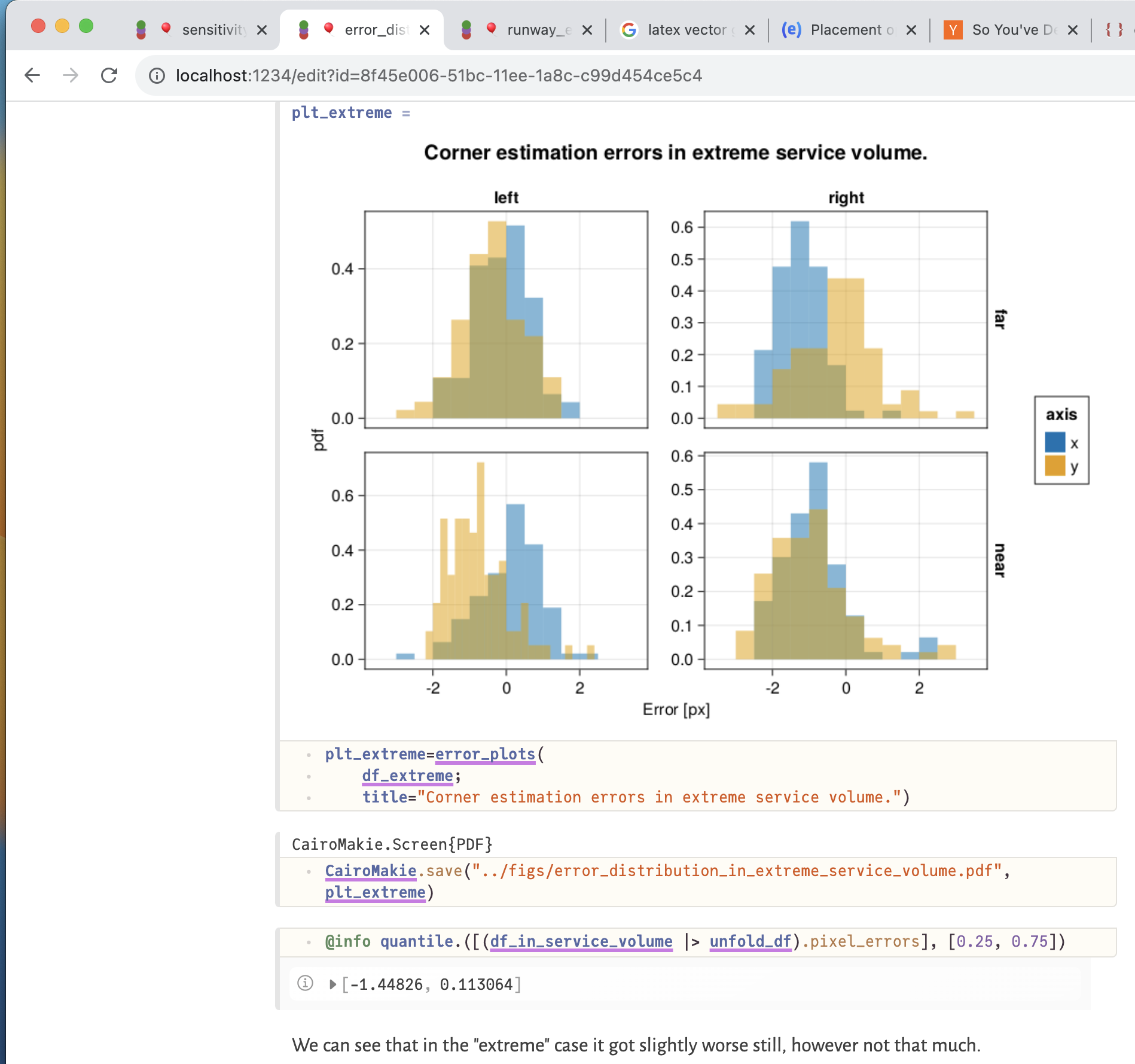
Pluto notebooks can be found in the notebooks directory. We provide two noteworthy notebooks, one for computing the empirical error distributions and correlations, and one presenting some of the theoretical sensitivity analysis.