| Documentation |
|---|
  |
| Build Status |
| Contacts |
 |
 |
 |
| Citation |
 |
A CPU and GPU research software for the numerical solution of a system of arbitrary conservation laws using continuous spectral elements and finite differences in 1D, 2D, 3D. DISCLAIMER: this will always be WIP! Contact us to join the team of developers!
Suggested Julia version: 1.10.0
If you use Jexpresso please drop us a line to let us know. We'd like to add a link to your paper or work on this page.
Please cite Jexpresso using:
@misc{tissaoui2024,
      title={Efficient Spectral Element Method for the Euler Equations on Unbounded Domains in Multiple Dimensions},
      author={Yassine Tissaoui and James F. Kelly and Simone Marras},
      year={2024},
      eprint={2401.05624},
      archivePrefix={arXiv},
      primaryClass={math.NA}
}
Jexpresso uses arbitrarily high-order (3rd and above) continuous spectral elements to solve
where the vectors
The Julia package DifferentialEquations.jl is used for time discretization and stepping.
In order, we provide tests and results for the following equations:
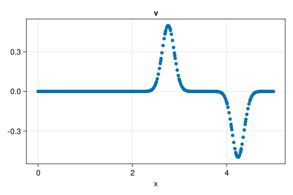
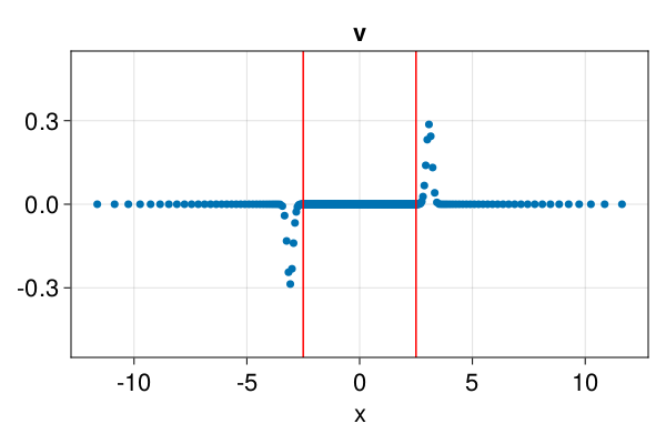
- 1D wave equation:
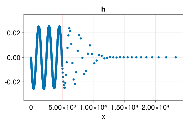
2: 1D shallow water:
where
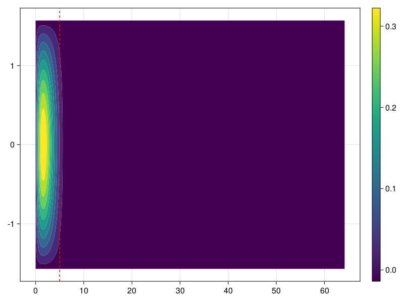
- 2D Helmholtz:
for a constant value of
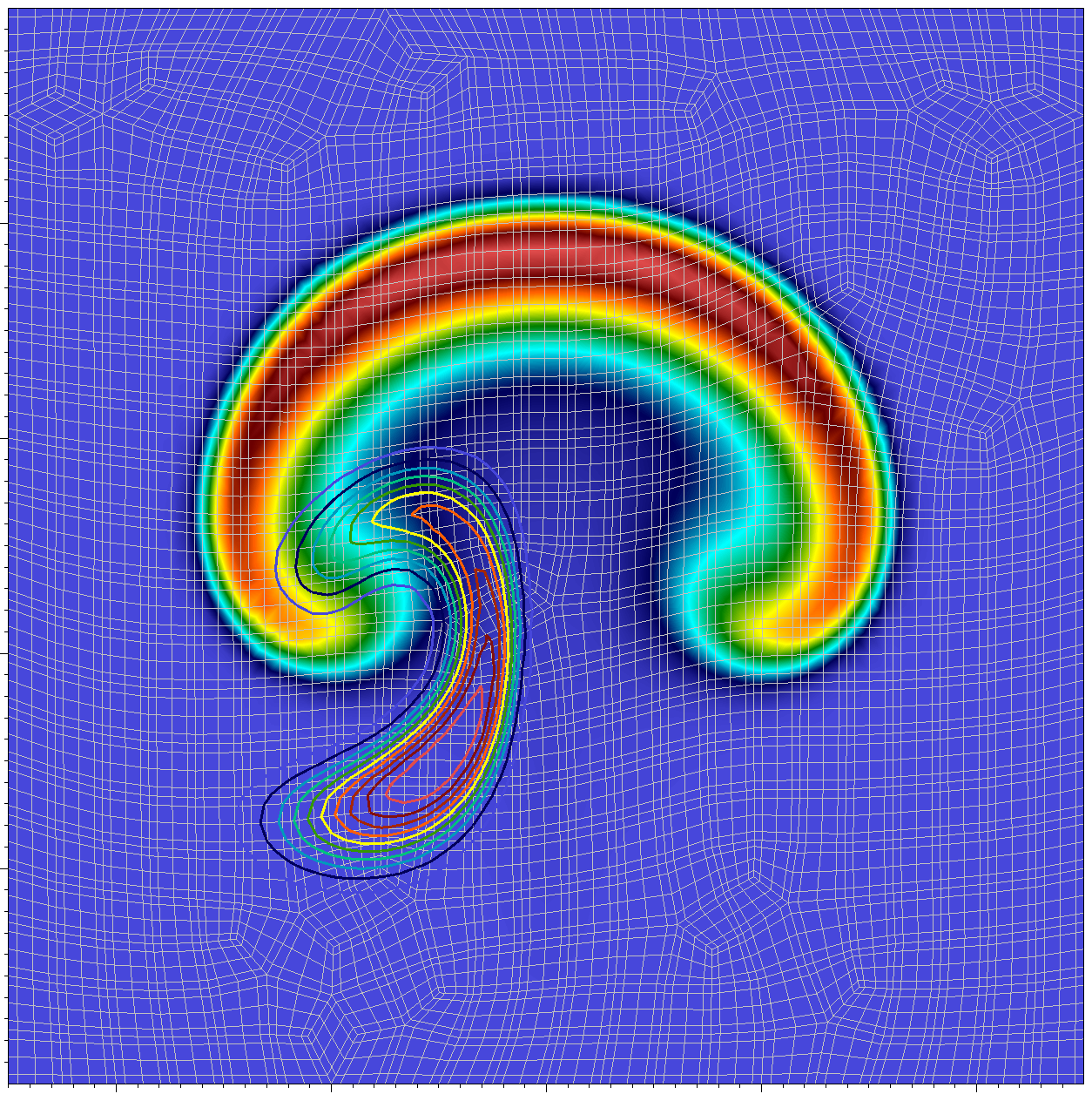
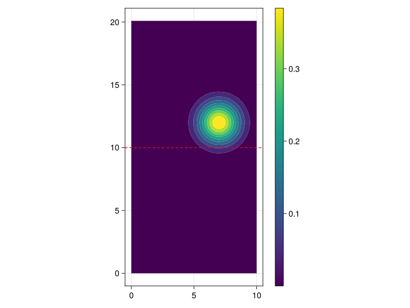
- 2D scalar advection-diffusion:
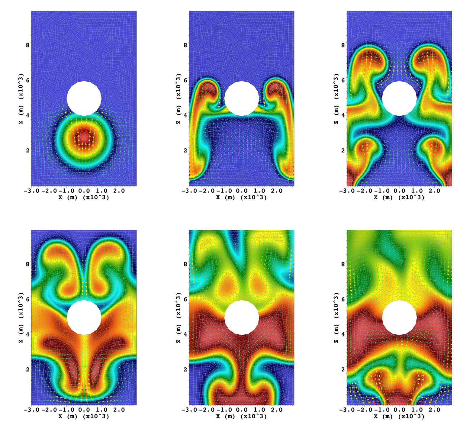
- 2D Euler equations of compressible flows with gravity and N passive chemicals
$c_i, \forall i=1,...,N$
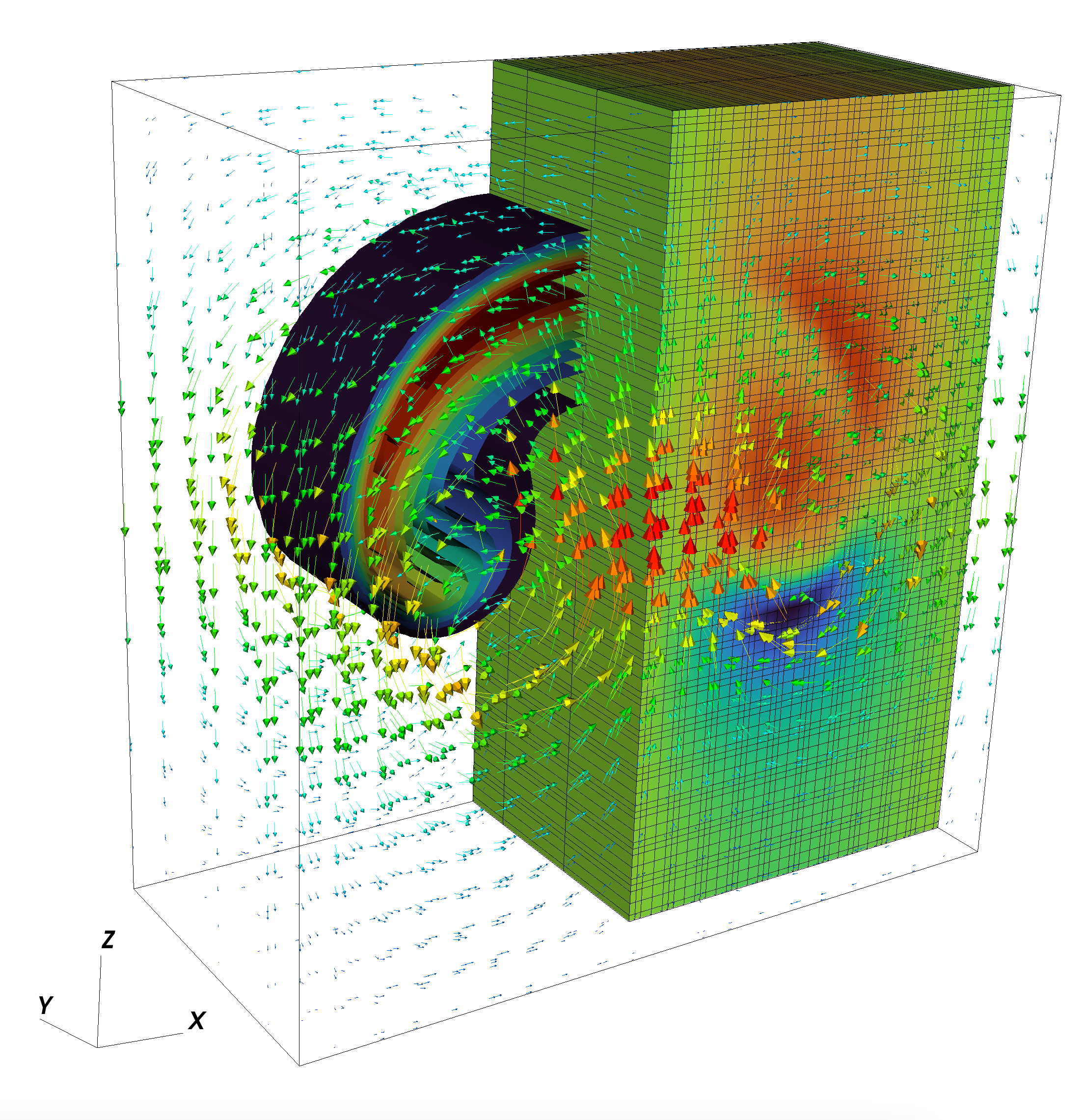
- 3D Euler equations of compressible flows with gravity
If you are interested in contributing, please get in touch: Simone Marras, Yassine Tissaoui
To install and run the code assume Julia 1.10.0
After cloning Jexpresso do the following:
>> cd $JEXPRESSO_HOME
>> julia --project=.
If on Apple, add Metal to the dependencies and continue to point 2:
1.apple
julia> ]
pkg> add Metal
pkg> instantiate
pkg> precompile
Notice that points 1. and 2. are for all, but 1.apple is required only for Apple users.
To run Jexpresso, do as follows:
Push problem name to ARGS You need to do this only when you run a new problem
julia> push!(empty!(ARGS), EQUATIONS::String, EQUATIONS_CASE_NAME::String);
julia> include("./src/Jexpresso.jl")- PROBLEM_NAME is the name of your problem directory as $JEXPRESSO/problems/equations/problem_name
- PROBLEM_CASE_NAME is the name of the subdirectory containing the specific setup that you want to run:
The path would look like
$JEXPRESSO/problems/equations/PROBLEM_NAME/PROBLEM_CASE_NAME
Example 1: to solve the 2D Euler equations with buyoancy and two passive tracers defined in problems/equations/CompEuler/thetaTracers you would do the following:
julia> push!(empty!(ARGS), "CompEuler", "thetaTracers");
julia> include("./src/Jexpresso.jl")
Example 2: to solve the 3D Euler equations with buyoancy defined in problems/equations/CompEuler/3d you would do the following:
julia> push!(empty!(ARGS), "CompEuler", "3d");
julia> include("./src/Jexpresso.jl")
Example 3: to solve the 2D Euler equations leading to a density current defined in problems/equations/CompEuler/dc you would do the following:
julia> push!(empty!(ARGS), "CompEuler", "dc");
julia> include("./src/Jexpresso.jl")
Example 4: to solve the 1D wave equation defined in problems/equations/CompEuler/wave1d you would do the following:
julia> push!(empty!(ARGS), "CompEuler", "wave1d");
julia> include("./src/Jexpresso.jl")
For ready to run tests, there are the currently available equations names:
- CompEuler (option with total energy and theta formulation)
The code is designed to create any system of conservsation laws. See CompEuler/case1 to see an example of each file. Details will be given in the documentation (still WIP). Write us if you need help.
More are already implemented but currently only in individual branches. They will be added to master after proper testing.
This section contains instructions to run all of the test cases presented in
@article{tissaoui2024,
  author = {Y. Tissaoui and J. F. Kelly and S. Marras}
  title = {Efficient Spectral Element Method for the Euler Equations on Unbounded Domains in Multiple Dimensions},
  url = {https://arxiv.org/abs/2401.05624},
  year = {2024},
  journal = {arXiv:2401.05624 [math.NA]},
}
Test 1: 1D wave equation with Laguerre semi-infinite element absorbing layers
The problem is defined in problems/CompEuler/wave1d_lag and by default output will be written to output/CompEuler/wave1d_lag. To solve this problem run the following commands from the Julia command line:
julia> push!(empty!(ARGS), "CompEuler", "wave1d_lag");
julia> include("./src/Jexpresso.jl")
Test 2: 1D wave train for linearized shallow water equations
The problem is defined in problems/equations/AdvDiff/Wave_Train and by default output will be written to output/AdvDiff/Wave_Train. To solve this problem run the following commands from the Julia command line:
julia> push!(empty!(ARGS), "AdvDiff", "Wave_Train");
julia> include("./src/Jexpresso.jl")
Test 3: 2D advection-diffusion equation
The problem is defined in problems/equations/AdvDiff/2D_laguerre and by default output will be written to output/AdvDiff/2D_laguerre. To solve this problem run the following commands from the Julia command line:
julia> push!(empty!(ARGS), "AdvDiff", "2D_laguerre");
julia> include("./src/Jexpresso.jl")
Test 4: 2D Helmholtz equation
The problem is defined in problems/equations/Helmholtz/case1 and by default output will be written to output/Helmholtz/case1. To solve this problem run the following commands from the Julia command line:
julia> push!(empty!(ARGS), "Helmholtz", "case1");
julia> include("./src/Jexpresso.jl")
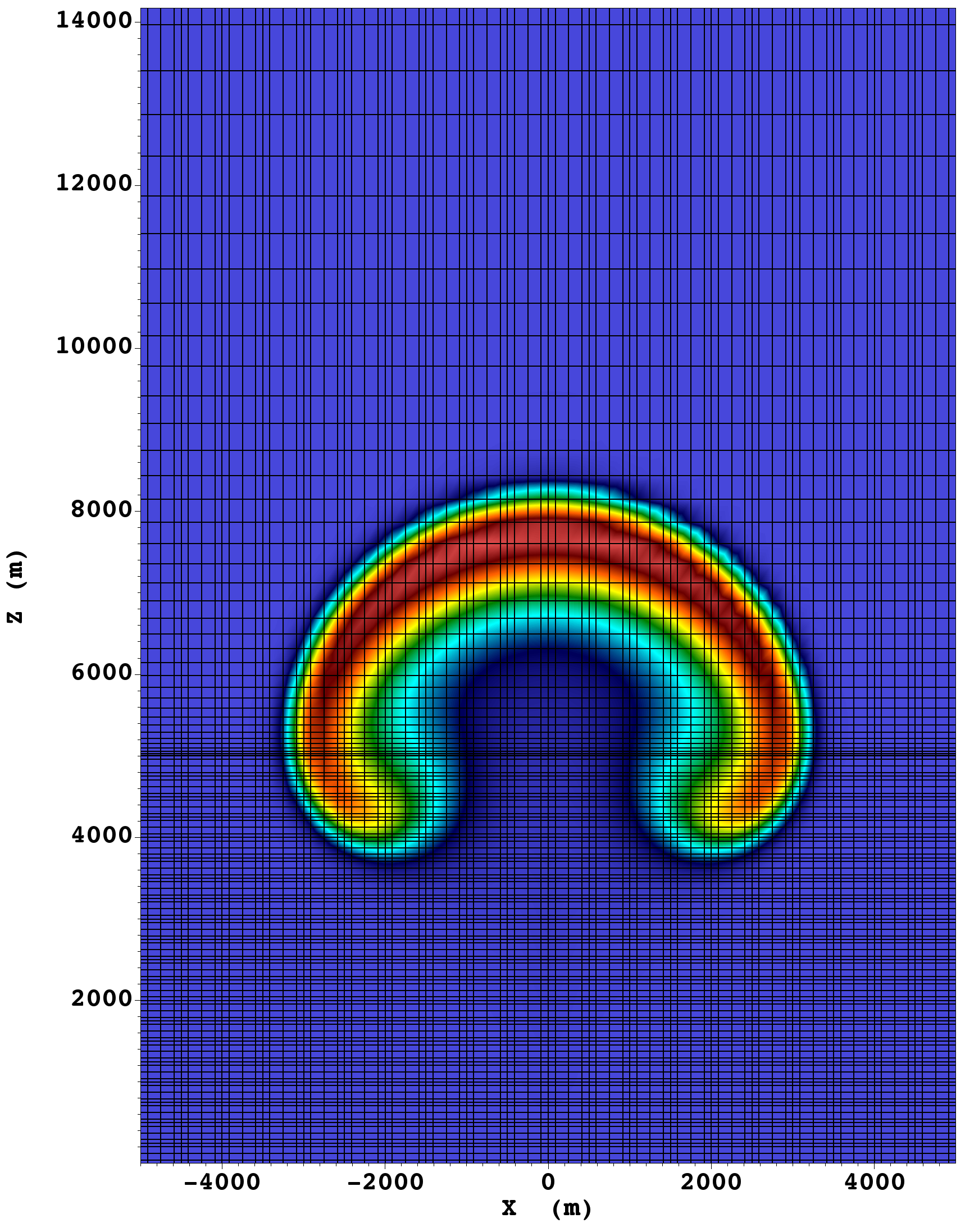
Test 5: Rising thermal bubble
The problem is defined in problems/equations/CompEuler/theta_laguerre and by default output will be written to output/CompEuler/theta_laguerre. To solve this problem run the following commands from the Julia command line:
julia> push!(empty!(ARGS), "CompEuler", "theta_laguerre");
julia> include("./src/Jexpresso.jl")
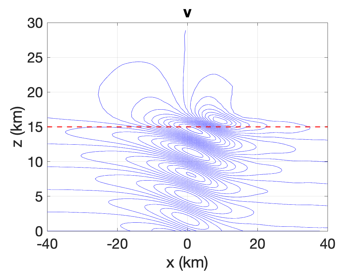
Test 6: Hydrostatic linear mountain waves
The problem is defined in problems/equations/CompEuler/HSmount_Lag_working and by default output will be written to output/CompEuler/HSmount_Lag_working. To solve this problem run the following commands from the Julia command line:
julia> push!(empty!(ARGS), "CompEuler", "HSmount_Lag_working");
julia> include("./src/Jexpresso.jl")Files can be written to VTK (recommended) or png. For the png plots, we use Makie. If you want to use a different package, modify ./src/io/plotting/jplots.jl accordinly.
For non-periodic 2D tests, the output can also be written to VTK files by setting the value "vtk" for the usier_input key :outformat

