WORK IN PROGRESS

tree-annotation

R scripts for annotation and exploration of protein phylogenetic trees and annotation of organism trees with phyletic patterns based on .

Features

Tree annotation

Annotation of nodes by tip-associated information by traversing along to the last ancestor
Manual annotation
Annotation of organism tree with occurence phyletic pattern from gene tree with grouping and taxonomic information

Tree visualization

One code line plotting with annotations from columns
- branch color
- tip text
- bar plots
- internal and external labels
- highlights
- bootstrap information
Flexible adjustment of taxonomic annotation
Linking taxa by sharing same property in a column
Visualization of domain architecture and genome context data
Visualization of trees with phyletic patterns at specified taxonomic prescision

Requirements

Make sure to install

library(tidyr)
library(dplyr)
library(readr)
library(data.table)
library(ggplot2)
library(treeio)
library(ggtree)
library(gggenes)
library(ape)
library(ggtreeExtra)
library(ggnewscale)

To install ggtree run in the R console

if (!require("BiocManager", quietly = TRUE))
    install.packages("BiocManager")

BiocManager::install("ggtree")

To install ggtreeExtra run

if (!require("BiocManager", quietly = TRUE))
    install.packages("BiocManager")

BiocManager::install("ggtreeExtra")

For the rest try

install.packages(package)

Usage

Currently, this tool is designed for working with data produced by tool. Perhaps in the future it will become more flexible.

Preparation

Load functions from tree_annotation.R and plot_tree.R

source('[path to tree_annotation.R]')
source('[path to plot_tree.R]')

Set working directory to directory with your data:

setwd('[path to your data]')

Load data

# protein tree
tree <- read.iqtree(file="tree.contree")

# annotation dataframe
annotation <- read.csv("filtered_clustered.csv")

# load the annotation data of filtered but not clustered hits (for the bacterial tree with phyletic pattern)
filtered_data <- read.csv("filtered_hits.csv")[, c('ID', 'assembly', 'taxid')]

# load the cluster data. which protein inherits properties from which representative
cluster_data <- read.csv("cluster_dict.csv")

# load the domain data.list of domains: which molecule they belong, domain name, start & end coordinates
domain_data <- read.csv("domains.csv")

# load genome context data
context_data <- read_context_data("genome_context.csv")  # working directory should contain "genome_context.csv" file

# LOAD SPECIES TREES AND ANNOTATIONS
org_tree_full <- read.tree(file="org_trees/org_tree_full.nwk")
org_tree_genus <- read.tree(file="org_trees/org_tree_genus.nwk")
org_tree_family <- read.tree(file="org_trees/org_tree_family.nwk")
org_tree_order <- read.tree(file="org_trees/org_tree_order.nwk")
org_tree_class <- read.tree(file="org_trees/org_tree_class.nwk")
org_tree_phylum <- read.tree(file="org_trees/org_tree_phylum.nwk")

org_tree_data <- read_delim("org_trees/org_tree_full_data.csv", delim=';')

Tweak your data if you need For example, replace "Candidatus" to "C." in org_tree_data

library('stringr')
org_tree_data$name <- str_replace(org_tree_data$name, "Candidatus", "C.")

Annotate the tree with data

tree <- annotate_tree(tree, annotation)

Tree exploration

Basics

For the most basic tree run

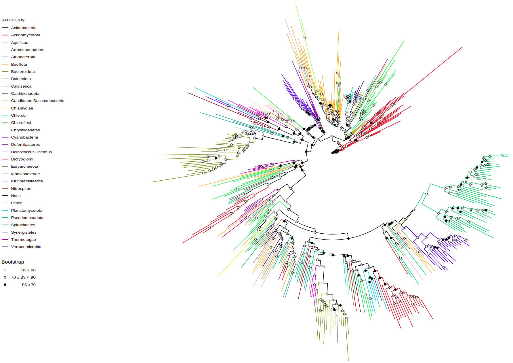
plot_tree(tree, filename="tree-base.svg", width=50, height=50)

By default it has circular layout, colored by taxonomy (phyla), and shows bootstrap values. These parameters are tweakable and additional annotations can be added.

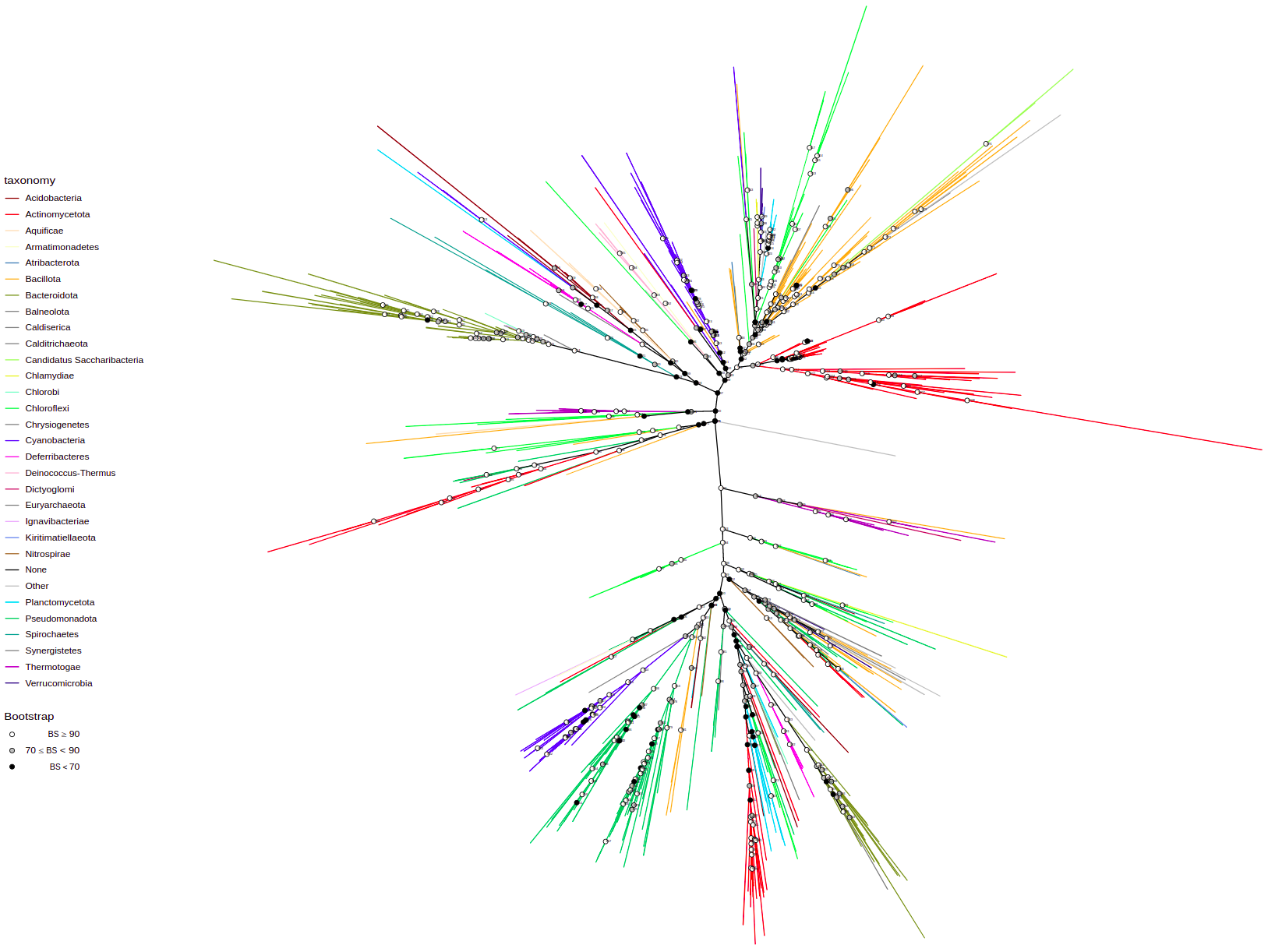
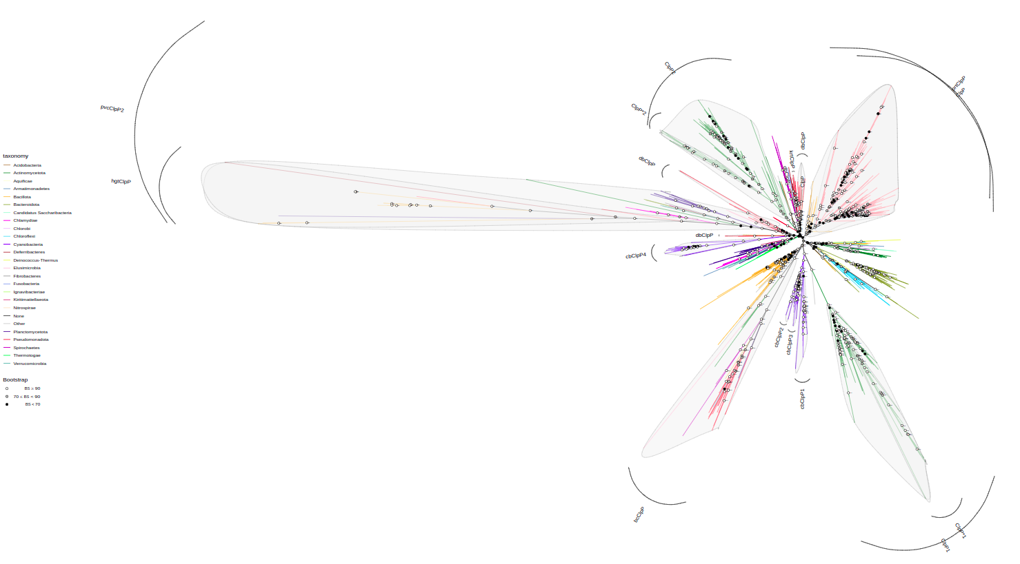
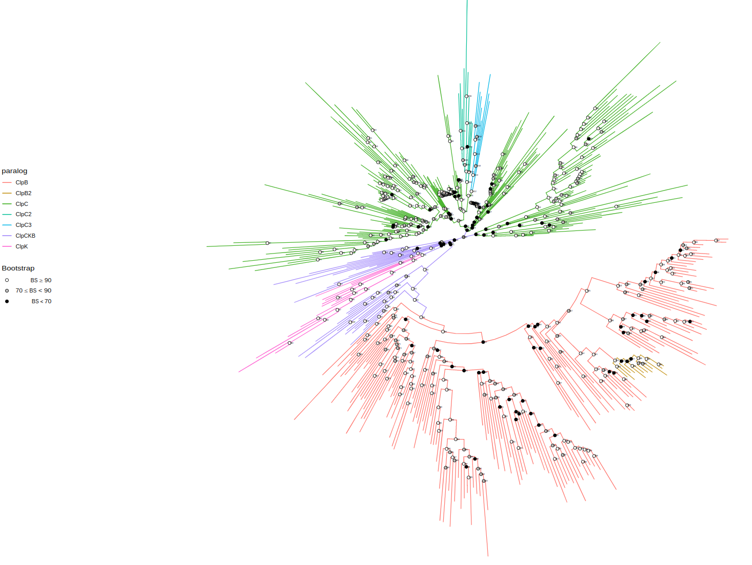
You can change tree layout using layout parameter. Available options: "circular", "rectangular", "equal_angle", "inward_circular".

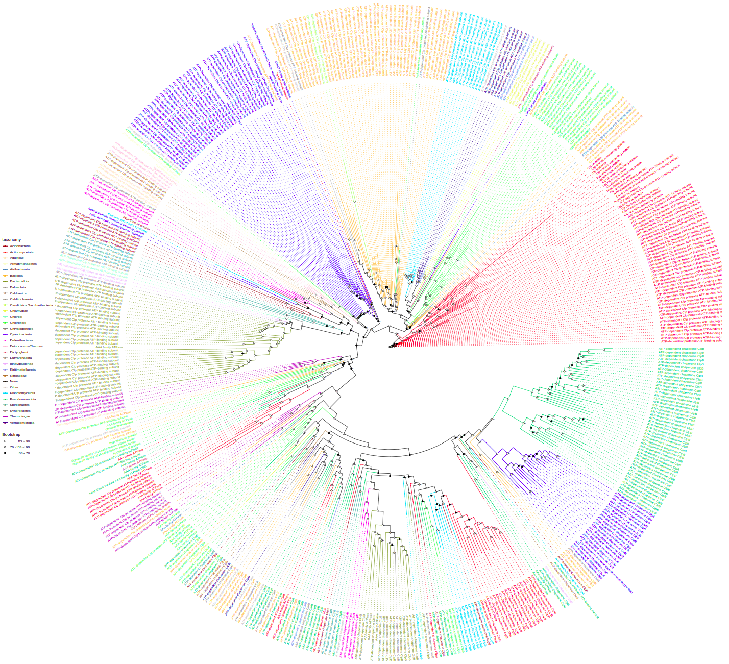
plot_tree(tree, layout="equal_angle", filename="equal_angle.svg", width=50, height=50)

You can label tree tips by tips parameter by different data associated with the tree, e.g. "gene", "product", "species", and so on.

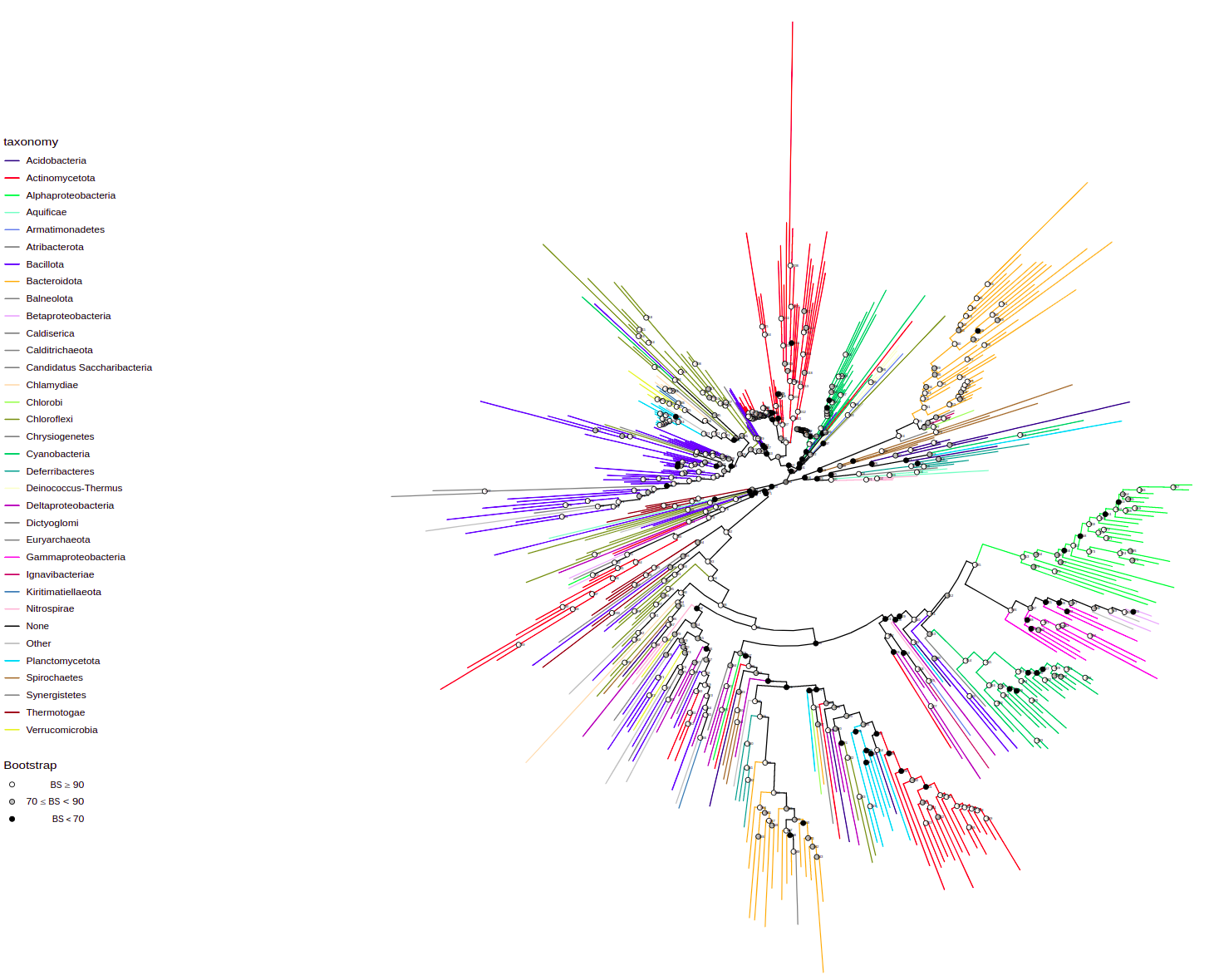
plot_tree(tree, tips="product", filename="tree-base-product.svg", width=75, height=75)

Adjustment of taxonomic annotation

To annotate some taxa on a lower taxonomic level use tax_expand parameter that contains taxon or vector of taxa that should be annotated at higher pescision. Here, we annotate Pseudomonadota (these are Proteobacteria) at the level of class

plot_tree(tree, tax_expand="Pseudomonadota", 
          filename="tree-expanded.svg", width=50, height=50)

Also you can specify the taxon, you want to start the annotation from by tax_start parameter

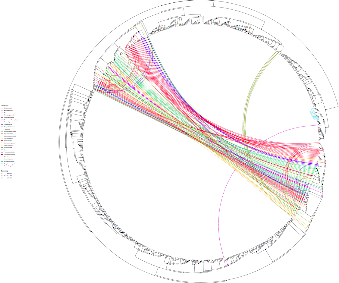
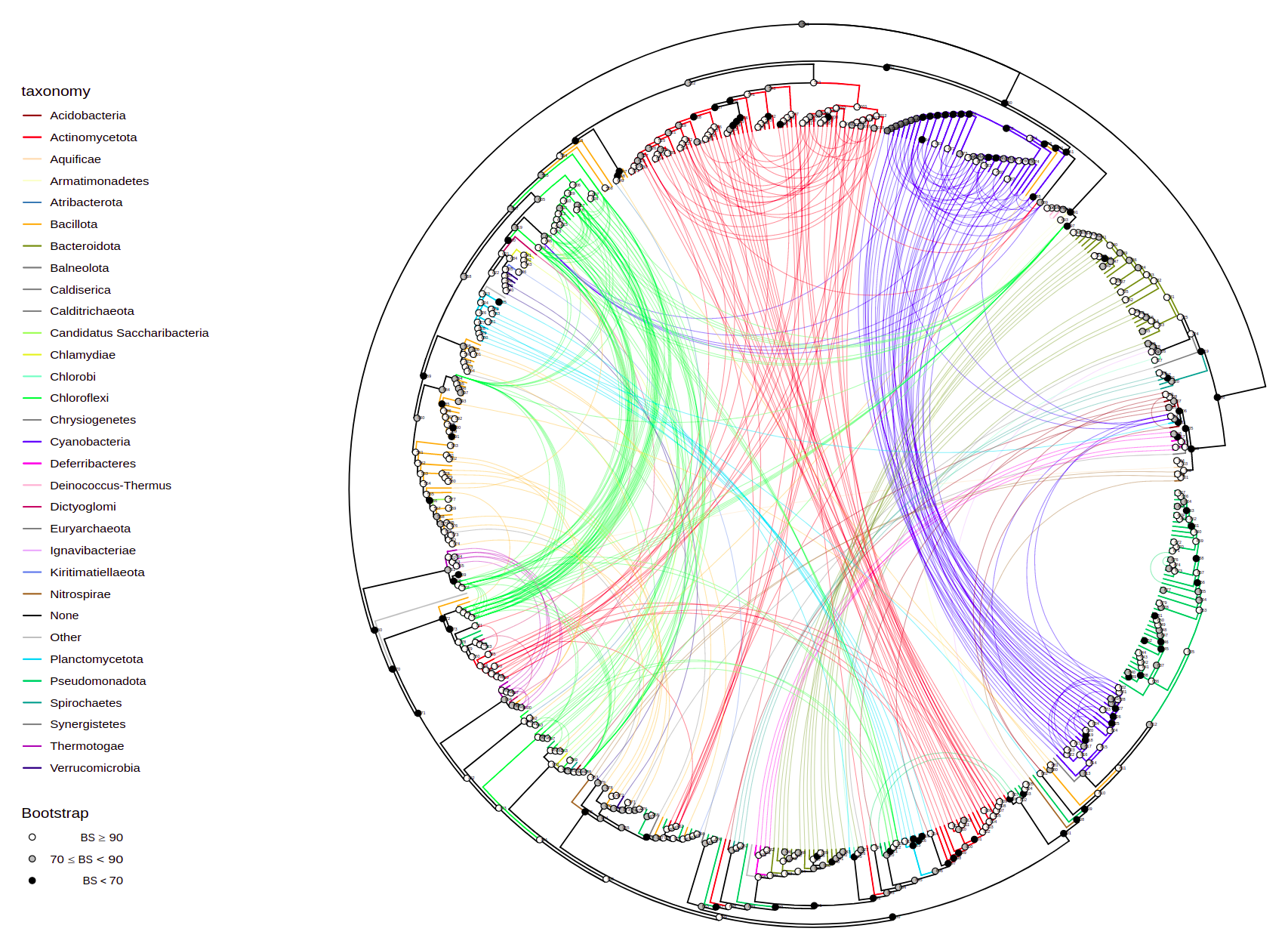
plot_tree(tree, layout="inward_circular", taxalink=T, branch_length='none', tips="gene",
          tax_start="Actinomycetota", tax_expand=c("Actinomycetota", "Actinomycetes"),
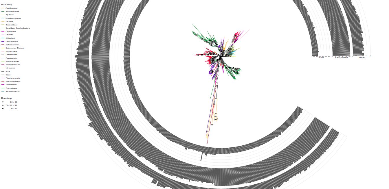
          width=100, height=100, filename="tree-taxalink-Act.svg")

Annotations

Barplots

You can plot quantitative information from columns by bars parameter

plot_tree(tree, filename="tree-bars.svg", bars=c("length", "query_coverage", "identity"), width=75, height=75)

Highlight and outer labels

Use highlight parameter to highlight branches by values in a column Use label_out parameter to make outer labels branches by values in a column

plot_tree(tree, highlight="paralog_anc", label_out="paralog_anc", bootstrap=F, 
          width=150, height=150, filename="tree-paralogs-HL.svg")

Inner labels

Use label to label nodes by value in a column

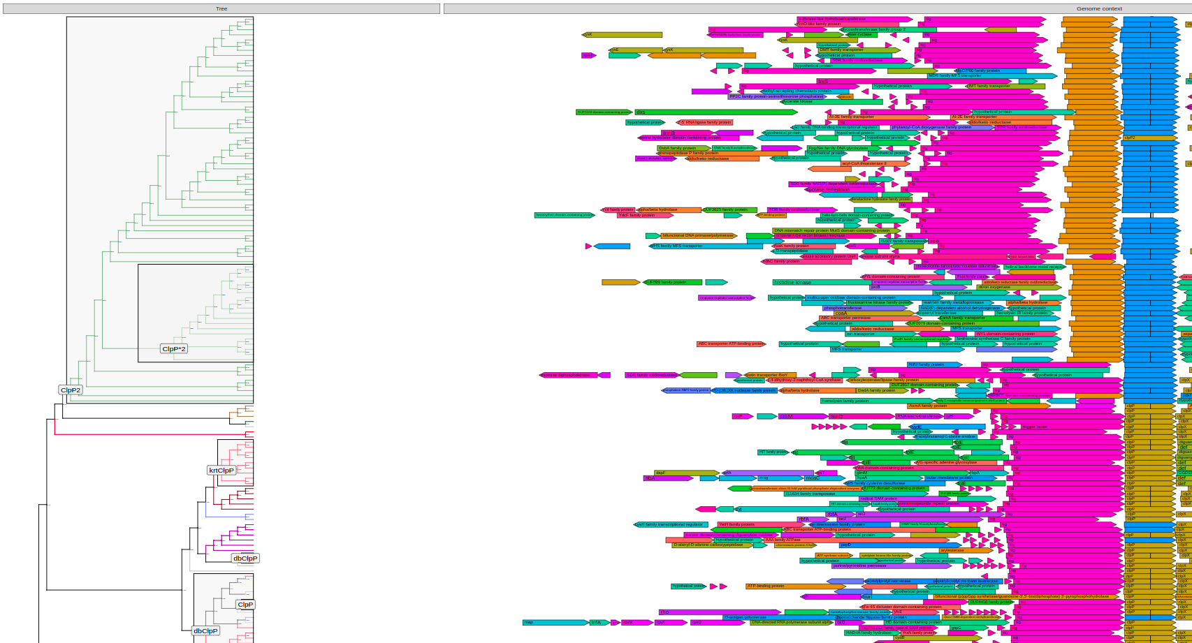
plot_tree(tree, label="paralog_anc", highlight="paralog_anc",context=context_data,
          layout="rectangular", branch_length="none", bootstrap=F, legend='none', # <-- params to make it not brake
          filename="tree-context-para.svg", height=200)

Rerooting

Depending on your observations you might want to reroot the tree using root() function provided by ggtree

tree = root(tree, node=697)

Taxalink

Link tips that have the same "assembly" value (what genome they are encoded in). To be custom in the future

plot_tree(tree, layout="inward_circular", taxalink=T, branch_length='none',
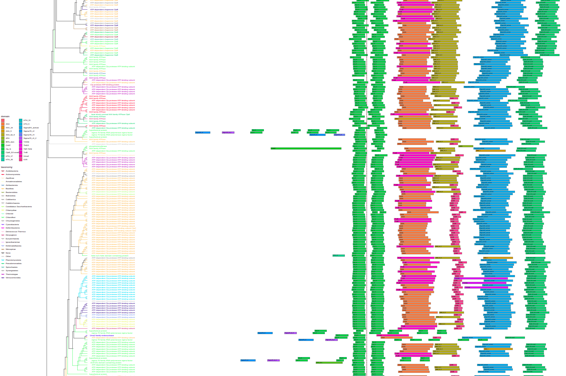
          width=50, height=33, filename="tree-taxalink.svg")

Domain architecture

plot_tree(tree, domains=domain_data, tips="product", 
          layout="rectangular", branch_length="none", bootstrap=F,   # <-- params to make it not brake
          filename="tree-domains.svg", height=200)

Genome context

plot_tree(tree, context=context_data, tips="product", 
          layout="rectangular", branch_length="none", bootstrap=F, legend='none',  # <-- params to make it not brake
          filename="tree-context.svg", height=200)

Assign paralogs

paralog_df = data.frame(
  node    = c(798,    690,     698,     760,    798,    778,    1002,    1012,  824), 
  paralog = c("ClpB", "ClpC", "ClpC", "ClpCKB", "ClpB", "ClpK", "ClpC2", "ClpC3", "ClpB2")
)
tree <- assign_paralogs(tree, "ClpCKB", paralog_df)

plot_tree(tree, color="paralog",
          width=50, height=50, filename="tree-paralogs.svg")

Organism tree annotation

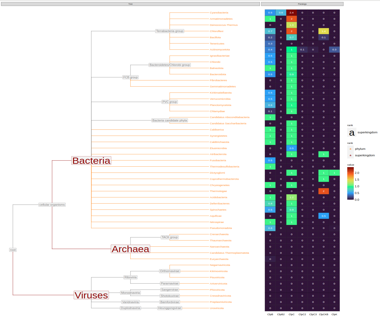
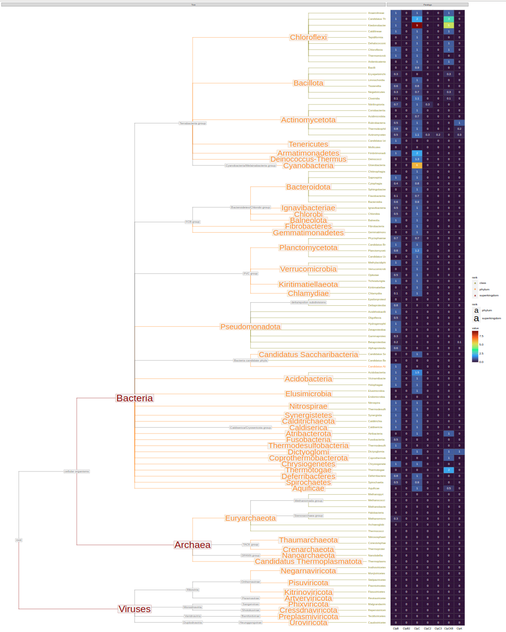
Once paralogs are assigned, you can annotate organism trees

species = annotate_org_tree(org_tree_full, org_data_full, tree)

phylum = copy_annotation(org_tree_family, org_tree_full_a)
class = copy_annotation(org_tree_class, org_tree_full_a)
order = copy_annotation(org_tree_class, org_tree_full_a)
family = copy_annotation(org_tree_class, org_tree_full_a)
genus = copy_annotation(org_tree_class, org_tree_full_a)

Organism tree plotting

And plot them at different taxonomic ranks

plot_org_tree(phylum, filename='org_tree_phylum.svg')

plot_org_tree(class, filename='org_tree_class.svg')

stovc/tree-annotation