A neural network model designed for multi-channel temporal signals. The Masked Conditional Neural Networks (MCLNN) is inspired by spectrograms and the use of filterbanks in signal analysis. It has been evaluated on sound. However, the model is general enough to be used for any multi-channel temporal signal. This work also introduces the Conditional Neural Networks (CLNN) inspired by the Conditional Restricted Boltzamann Machine (CRBM) [1]. The CLNN is the main structure for the MCLNN operation.
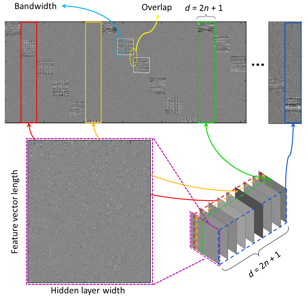
The MCLNN allows inferring the middle frame of a window of frames, in a temporal signal, conditioned on n preceeding and n succeeding frames. The mask enforces a systematic sparsness that follows a filterbank-like pattern and it automates the mixing-and-matching between different feature combinations at the input, analgous to the manual hand-crafting of features.
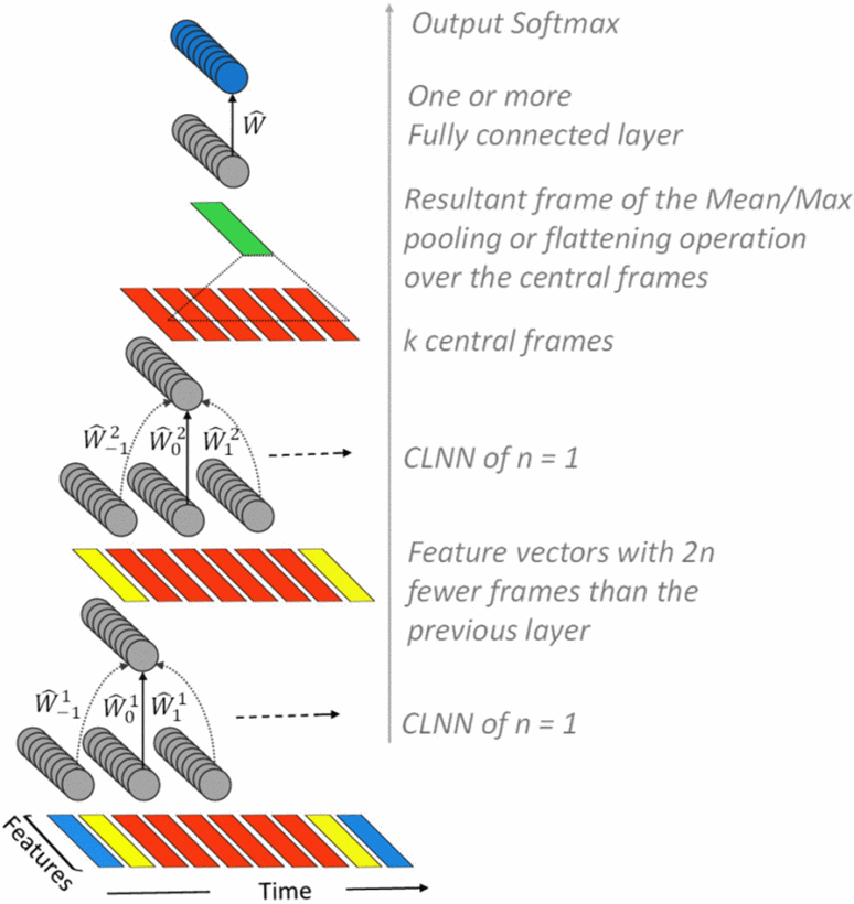
The below figure shows a network having two CLNN layers. The CLNN is used as a structure for the MCLNN.
The below figure shows a weight matrix with the enforced filterbank-like behavior enforced over the weights of a single temporal instance using a systematic controlled sparsness.
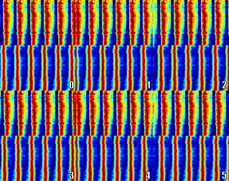
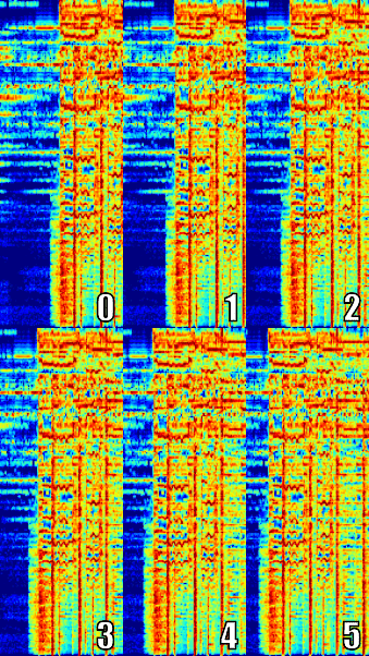
The below figures show 30 segments of a spectrogram as an input (colored) and their corresponding output (grayscale) from an MCLNN before applying any activation function. The spectrogram shown is a frequency-wise concatenation between a logarithmic 60-bins mel-scaled spectrogram and its delta (left figure) and a 256-bin spectrogram of the Ballroom dataset (right figure).
A visualization of MCLNN weights for sample hidden nodes
-
Frameworks:
- CUDA release 7.5, v7.5.17
-
Python (version 2.7.11) environment and packages:
- Keras 1.0.8
- Theano 0.8.2
- memory_profiler 0.52.0
- numpy 1.9.2
- scipy 1.0.1
- h5py 2.8.0
- matplotlib 2.2.3
- scikit_learn 0.19.2
-
Sound related:
- FFmpeg version N-81489-ga37e6dd (built with gcc 5.4.0)
- librosa 0.4.0
- muda 0.2.0
The MCLNN code requires two .hdf5 files, one containing the samples and another of the indices.
A single file containing the intermediate representation (e.g. spectrograms for sound) of all the files of a single dataset. Samples are the complete clips (segmentation is handled within the MCLNN code). Samples are ordered by their category name in ascending order, similarly samples within a category are ordered by their name. Refer to the dataset_transformer folder for more details.
These are primarily 3 files, training, testing and validation. Each of the indices files hold the indices of the samples following their location in the Samples.hdf5. These files can be generated as many times as the number of cross-validation operation, i.e. 10-fold cross-validation will have 30 index files generated, where every triple are: training.hdf5 containing 8-folds for training, validation.hdf5 having 1-fold for validation and testing.hdf5 with 1-fold for testing. Folds are shuffled across the n-fold cross-validation. Refer to the index_generator folder for more details.
Below are the most important configuration required by the MCLNN categorized into subsections.
The parent folder for the training/validation/testing .hdf5 index files for the n-folds and the Dataset.hdf5 file generated by the transformer.
PARENT_PATH = 'parent/folder/path/'
The main .hdf5 file containing the dataset processed samples, e.g. spectrograms.
DATASET_FILE_PATH = os.path.join(PARENT_PATH, 'Dataset.hdf5')The dataset name and the number of folds are used to name the index, standardization, weights and visualization folders as below. So make sure the index folder is named with the convention: 'datasetname_folds_count_index', e.g. ESC10_folds_5_index.
The the visualization folder stores the images for weights and activations, if any of the visualization flags is enabled.
DATASET_NAME = 'datasetname'
CROSS_VALIDATION_FOLDS_COUNT = 5
COMMON_PATH_NAME = os.path.join(PARENT_PATH, DATASET_NAME + '_folds_' + str(CROSS_VALIDATION_FOLDS_COUNT))

INDEX_PATH = COMMON_PATH_NAME + '_index'
STANDARDIZATION_PATH = COMMON_PATH_NAME + '_standardization'
ALL_FOLDS_WEIGHTS_PATH = COMMON_PATH_NAME + '_weights'
VISUALIZATION_PARENT_PATH = COMMON_PATH_NAME + '_visualization'The step size specifies the number of overlapping frames between consecutive segments. This number affects the processing stage of the segments present in the samples .hdf5 file. It also affects the number of samples that will be available for training.
# overlap between segments is q minus step_size
STEP_SIZE = 1
Number of epochs or wait count, will take over to stop the model's training.
# maximum number of epochs
NB_EPOCH = 2000

# early stopping count
WAIT_COUNT = 50
Track the validation accuracy or loss for the early stopping.
# track the validation accuracy or loss for the stopping criterion : 'val_acc' or 'val_loss'
STOPPING_CRITERION = 'val_acc'
Load pretrained model or start training from scratch. If this flag is enabled, pre-trained weights should be present in the weights parent folder (ALL_FOLDS_WEIGHTS_PATH).
# use pretrained weights or train a model from scratch
USE_PRETRAINED_WEIGHTS = False # True or FalseNumber of classes under consideration
NB_CLASSES = 10 # number of classesThe names of the classes. These are the names used for the confusion matrix.
CLASS_NAMES = ['DB', 'Ra', 'SW', 'BC', 'CT', 'PS', 'He', 'Ch', 'Ro', 'FC']Below are the hyperparameters for each layer of a five layers model. For each new layer of a deeper model, append its hyperparameters to the relevant list below. Note: all lists should be equal in length, following the number of layers in a model.
# dropout at the input of each layer
DROPOUT = [0.01, 0.5, 0.5, 0.5, 0.1]

# hidden nodes for each layer, Note: the last element is the number of classes under consideration.
HIDDEN_NODES_LIST = [300, 200, 100, 100, NB_CLASSES]

# initialization at each layer.
WEIGHT_INITIALIZATION = ['he_normal', 'he_normal', 'glorot_uniform', 'glorot_uniform', 'glorot_uniform']
The count of MCLNN and Dense layers
# Model layers
MCLNN_LAYER_COUNT = 2  # number of MCLNN layers
DENSE_LAYER_COUNT = 2  # number of Dense layers
MCLNN specific hyperparameters
The order for a two-layered MCLNN. The first MCLNN layer has an order of 17 and the second has an order of 15.
# the order for each layer
LAYERS_ORDER_LIST = [17, 15]
Disable/Enable the mask of each layer. "False" converts the layer to CLNN and the mask parameters (bandwithd and overlap) are ignored.
LAYER_IS_MASKED = [True, True] # True: MCLNN, False: CLNN (Bandwidth and Overlap are ignored in this case)
The Mask Bandwidth of a two-layered MCLNN. The first layer has a bandwithd of 20 and the second layer has a bandwidth of 5.
# the consecutive features enabled at the input for each layer
MASK_BANDWIDTH = [20, 5]
The Mask Overlap of a two-layred MCLNN. The first layer has an overlap of -5 and the second layer has an overlap of 3.
# the overlap of observation between a hidden node and another for each layer
MASK_OVERLAP = [-5, 3]
The extra frames for the single-dimensional temporal pooling. Note: the middle frame is add to the below value by default.
# the k extra excluding the middle frame (middle frame is included by default)
EXTRA_FRAMES = 40 The below flag allows saving the output of the first MCLNN layer of a model during the training stage. NOTE: this flag is for trial visualization only, it will affect the training. Accordingly, this flag should ALWAYS be disabled to train a proper model. (This has to do with prediction during training and the Learning_Phase flag used by Keras)
SAVE_SEGMENT_PREDICTION_IMAGE_PER_EPOCH = FalseThe indices of the segments to be saved if the SAVE_SEGMENT_PREDICTION_IMAGE_PER_EPOCH flag is enabled.
TRAIN_SEGMENT_INDEX = 500 # train segment index to plot during training
TEST_SEGMENT_INDEX = 500 # test segment index to plot during training
VALIDATION_SEGMENT_INDEX = 500 # validation segment index to plot during training
The below flag enables segments generation from the test data after training.
# store prediction images for segments of a specific clip of testing data
SAVE_TEST_SEGMENT_PREDICTION_IMAGE = True  # True or False
The start index of the test sample to generate the prediction for, together with the number of segments to generate. Note: SAVE_TEST_SEGMENT_PREDICTION_IMAGE should to enabled for the below parameters to take effect.
# index of starting segment to plot.
SAVE_TEST_SEGMENT_PREDICTION_INITIAL_SEGMENT_INDEX = 50  # used only if the SAVE_LAYER_OUTPUT_IMAGE is enabled

# number of segments to save after the starting segment.
SAVE_TEST_SEGMENT_PREDICTION_IMAGE_COUNT = 30  # used only if the SAVE_LAYER_OUTPUT_IMAGE is enabled
Visualize the weights affecting the hidden nodes at each MCLNN layer. The count specifies the number of hidden nodes to visiualize.
HIDDEN_NODES_SLICES_COUNT= 40 # weights visualization for n hidden nodesThe MCLNN has been evaluated using a range of datasets. The required configuration for each one is available in the configuration.py
We have created a separate repository for the prepossessing required for each dataset, please refer to them for more details.
| Dataset | MCLNN accuracy % |
|---|---|
| ESC10 | 85.5 |
| ESC10 augmented | 85.3 |
| ESC50 | 62.9 |
| ESC50 augmented | 66.6 |
| UrbanSound8k | 74.2 |
| YorNoise | 75.8 |
| Homburg | 61.5 |
| GTZAN | 85.0 |
| ISMIR2004 | 86.0 |
| Ballroom | 92.6 |
If you are using the MCLNN in your work please cite us as follows based on the dataset and the MCLNN architecture used:
GTZAN or ISMIR2004 music datasets and temporal signals other than sound.
Fady Medhat, David Chesmore, John Robinson, Masked Conditional Neural Networks for Audio Classification International Conference on Artificial Neural Networks and Machine Learning, ICANN 2017.
Ballroom music dataset - shallow MCLNN with long segments.
Fady Medhat, David Chesmore, John Robinson, Automatic Classification of Music Genre Using Masked Conditional Neural Networks, IEEE International Conference on Data Mining, ICDM, 2017.
Ballroom or Homburg music datasets - deep MCLNN with short segments.
Fady Medhat, David Chesmore, John Robinson, Music Genre Classification Using Masked Conditional Neural Networks, International Conference on Neural Information Processing, ICONIP, 2017.
Urbansound8k, YorNoise, ESC-10 and ESC-50 environmental sound datasets - shallow MCLNN with long segments.
Fady Medhat, David Chesmore and John Robinson, Recognition of Acoustic Events Using Masked Conditional Neural Networks, IEEE International Conference on Machine Learning and Applications, ICMLA, 2017.
ESC-10 environmental sound dataset - deep MCLNN with long segments.
Fady Medhat, David Chesmore and John Robinson, Environmental Sound Recognition Using Masked Conditional Neural Networks, Advanced Data Mining and Applications, ADMA, 2017.
YorNoise and UrbanSound8k environmental sound datasets - deep MCLNN with short segments.
Fady Medhat, David Chesmore and John Robinson, Masked Conditional Neural Networks for Environmental Sound Classification, Artificial Intelligence XXXIV. SGAI, 2017.
ESC-50 and ESC10 environmental sound datasets, CLNN vs MCLNN - deep MCLNN with short segments.
Fady Medhat, David Chesmore and John Robinson, Masked Conditional Neural Networks for Automatic Sound Events Recognition, IEEE International Conference on Data Science and Advanced Analytics, DSAA, 2017.
[1] G.W. Taylor, G.E. Hinton, S. Roweis, Modeling Human Motion Using Binary Latent Variables In: Advances in Neural Information Processing Systems, NIPS, 2006


