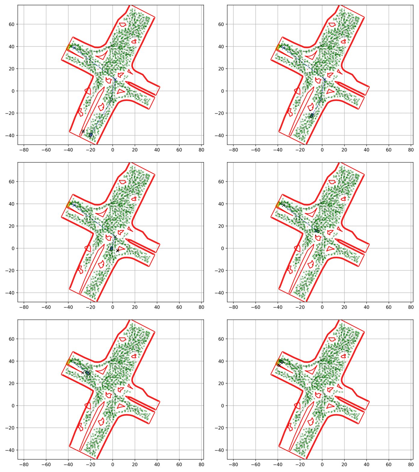
For the Planning and Decision-Making for Autonomous Robots course at ETH Zurich, I implemented the RRTx path-finding algorithm.
RRTx is different from other RRT algorithms like RRT* and RRT# as it is able to react to changes in the environment without needing to replan.
This was useful for my assignment where multiple agents (cars) needed to independently find paths to goals around the map. Cars might obstruct each other. To reduce the need for costly replanning from scratch, RRTx allows us to reuse the original calculated graph.
Furthermore, we are able to use RRTx as a "feedback control" policy, as the trajectory generated from RRTx will be with respect to the current position of the robot.
Below are gifs of the algorithm working in a static and a dynamic environment. Unfortunately the algorithm only works in the Docker environment specified for the assignment, so you would need to adapt the sample code to your specific use case.
It can be seen that the path (in blue) changes dynamically as the agent moves through it. It is formed by tracing nodes back to the goal position, and pruing (details in the path smoothing section).
The black points tracking the obstacles are the nearest obstacle to the vehicle, used as a heuristic for speed control.
The video can be seen on YouTube.
It can be seen that when agents detect that other agents (modelled as circles centered about the predicted center of other agents) would block their trajectories, they stop. So long as one agent has a viable path to the goal, no deconfliction is needed.
To save computation, agents only consider other agents in their front 180 degrees. You can observe this as dynamic obstacles appearing and disappearing as the agents turn around.
For more robust matching, agents could be programmed to detect blind corners (eg. around obstacles). This would allow for higher safe top speeds, or lower overall control efforts.
Points are sampled in a 2D coordinate space. Nodes are then stored in a Scipy KD-Tree for fast nearest-neighbor querying. This meant that it was not so easy to extend the state space to include a "heading" (angular) dimension, as angles wrap around, causing a different measure of distance compared to regular Euclidean coordinates. However, this issue could be fixed by just making the state space 4D: x, y, sin(theta), cos(theta).
In practice it was found that this made the algorithm more sample-inefficient, so it was dropped.
As it is assumed that static obstacles do not move, they are stored in a Shapely R-Tree for easier collision checking with a circle representing the vehicle. Dynamic obstacles are assumed to be other agents (and rather small in number), so they are stored in a simple Python list.
The beauty of RRTx is that if an obstacle is detected to intersect the future trajectory of an agent, the agent is able to re-plan around it, switching to a valid trajectory if it exists, or stopping if it doesnt. This removes the need for explicit deconfliction or right-of-way, although it is possible that with more complicated scenarios, some form of high-level deconfliction would be desirable or necessary.
Trajectories are initially very jagged, as they follow each randomly-sampled RRT node back to the goal. This is difficult for the vehicle to follow, so a path-smoothing heuristic is followed.
We check if a line without collision and with sufficient obstacle clearance can be drawn from one node to another node while skipping one or more intermediate nodes. If this is possible, the intermediate nodes are pruned.
This results in a much smoother path with more straight segments for vehicles to follow.
The vehicle in the exercise was a dynamic vehicle where only the acceleration of the vehicle and the rate of change of steering angle can be controlled. In this case we need two controllers: lateral (steering) and longitudinal (speed).
The Stanely controller was used. A good explanation is here. The original paper is also quite readable.
This controller calculates the desired steering angle with respect to the difference in the current steering angle, the current heading of the vehicle, and the heading of the closest point of the trajectory with respect to the front axle of the vehicle.
A PD controller is then used to give a control command to track the desired steering angle.
For speed control, three cost functions were implemented.
- A "lookahead" cost. Intuitively, a trajectory with larger angles closer to the vehicle should accrue a higher cost.
- A "deviation" cost. The larger the steering error or the deviation from the trajectory, the more the vehicle should slow down.
- A "clearance" cost. The closer the vehicle is to an obstacle, the slower it should travel. However, if the obstacle is parallel to the direction of travel of the vehicle, it should not slow the vehicle.
The costs are then added, and the desired vehicle speed is then: max(V_MIN, V_MAX-cost).
The code is in rrtx.py. Remember to take a look at the requirements in requirements.txt.
If you have any questions, do raise an issue or even a PR. If this helped you, do give a star!
