 |
|---|
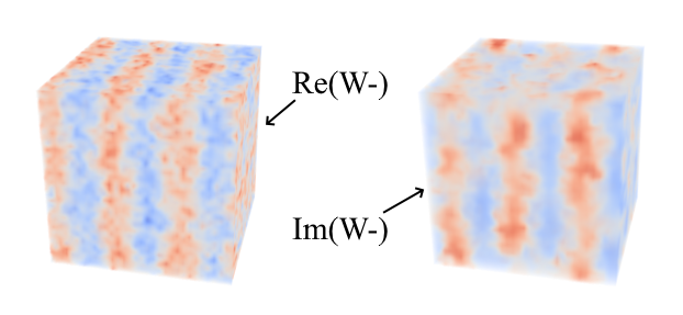
| Real and imaginary parts of W-(r) at Nbar=105, N=90, χN=12, m=32 and L=4.209. |
See https://www.tbeardsley.com/projects/lfts/clfts_gpu for a detailed discussion of this project.
CUDA Toolkit (https://developer.nvidia.com/cuda-toolkit/)
Two methods of compiling the program are available:
- comp.sh
A simple bash script to create a 'build' directory containing the compiled program code: clfts-gpu.
On a Linux system, run the bash script from the top directory via:
sh comp.sh
- CMake
CMakeLists.txt specifies the required commands for CMake to create (and run) Makefiles, which create a 'build' directory and compile the program code as: clfts-gpu.
From the top directory, run:
cmake -B build
cmake --build build
After compilation the executable file, clfts-gpu, resides in the 'build' directory. An input file must be supplied to the executable at the command line, examples of which are contained in the 'input_files' folder.
For example, from the top level of the directory tree, the program could be run via:
./build/clfts-gpu ./input_files/input
The input_files directory contains example input files that can be supplied to the program from the command line.
Line 1: N NA XeN zetaN C Ndt
Line 2: mx my mz Lx Ly Lz
Line 3: n_eq n_st n_smpl save_freq
Lines 4->(M+3): REAL[W-(r)] IMAG[W-(r)]
Lines (M+4)->(2M+3): REAL[W+(r)] IMAG[W+(r)]
Notes:
A real-space position r = (x,y,z) corresponds to a mesh point position r_m = (i,j,k), where i=0->mx-1, j=0->my-1 and k=0->mz-1 are integers. The elements of the fields, W-(r) and W+(r), are then written in ascending order of the row-major index: p = mx*(i*my+j)+k.
| Parameter | Type | Description |
|---|---|---|
| N | Integer | Number of monomers in a single polymer chain |
| NA | Integer | Number of monomers in the A-block of a polymer chain |
| XeN | Double | Interaction strength between A and B-type monomers |
| zetaN | Double | Compressibility factor, zeta, multiplied by N |
| C | Double | Square root of the invariant polymerisation index, Nbar |
| Ndt | Double | Size of the time step in the Langevin update of W-(r) |
| mx, my, mz | Integers | Number of mesh points in the x, y, and z dimensions of the simulation box |
| Lx, Ly, Lz | Doubles | Dimensions of the simulation box (in units of the polymer end-to-end length, R0) in the x, y, and z dimensions |
| n_eq | Integer | Number of langevin steps performed to equilibrate the system |
| n_st | Integer | Number of langevin steps performed after equilibration has ended, during which statistics are sampled |
| n_smpl | Integer | Number of steps between samples being taken in the statistics period |
| save_freq | Integer | Number of steps between saving outputs to file |
| M | Integer | Total number of mesh points (M = mx*my*mz), such that the proceeding 2*M lines of the file can hold the W-(r) and w+(r) fields to be loaded |
The state of the W-(r) and w+(r) fields at simulation step number <step_number> during the equilibration period. First three lines are simulation parameters so it can be used as an input file.
The state of the W-(r) and w+(r) fields at simulation step number <step_number> during the statistics gathering period. First three lines are simulation parameters so it can be used as an input file.
The state of the phi-(r) and phi+(r) fields at simulation step number <step_number> during the equilibration period.
The state of the phi-(r) and phi+(r) fields at simulation step number <step_number> during the statistics gathering period.
The spherically-averaged structure function at simulation step number <step_number> during the statistics gathering period.
The tools folder in the root directory contains a simple script for taking the first M lines of a w_<..><step_number> or phi<..>_<step_number> output file from the simulation, and creating a .vtk file that can be loaded into Paraview for visualisation as a volume plot. Note that the first M lines are used as they correspond to the W-(r) or phi-(r) fields, which are usually the ones of interest. The script could easily be edited to use lines M+1 to 2M in order to plot w+(r) or phi+(r) instead.
The script can be run from the command line as follows:
sh make_vtk.sh <path_to_file_to_visualise> <mx> <my> <mz>
where mx, my and mz are the number of grid points in the x, y and z-dimensions of the file being visualised.
The script's output file name will be the same as <path_to_file_to_visualise>, but with a .vtk extension.