CLP(B): Constraint Logic Programming over Boolean variables

CLP(B), Constraint Logic Programming over Boolean variables, is available in Scryer Prolog and SWI-Prolog as library(clpb).

This repository contains usage examples and tests of the library.

clpb.pdf is a shortened version of the library documentation, intended as supplementary lecture material.

Project page:

https://www.metalevel.at/clpb/

Using CLP(B) constraints

Many of the examples use DCG notation to describe lists of clauses. This lets you easily reason about the constraints that are being posted, change the order in which they are posted, and in general more conveniently experiment with CLP(B). In some examples, it is faster to post a single big conjunction instead of several smaller ones.

I recommend you start with the following examples:

knights_and_knaves.pl: Solution of several Boolean puzzles that appear in Raymond Smullyan's What Is the Name of this Book and Maurice Kraitchik's Mathematical Recreations. These examples and other logic puzzles are good starting points for learning more about CLP(B).
xor.pl: Verification of a digital circuit, expressing XOR with NAND gates:

This example uses universally quantified variables to express the output as a function of the input variables in residual goals.
matchsticks.pl: A puzzle involving matchsticks. See below for more information.
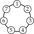
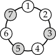
cycle_n.pl: Uses Boolean constraints to express independent sets and maximal independent sets (also called kernels) of the cycle graph C_N.

See below for more information about weighted solutions.
euler_172.pl: CLP(B) solution of Project Euler Problem 172: How many 18-digit numbers n (without leading zeros) are there such that no digit occurs more than three times in n?
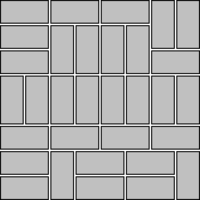
domino_tiling.pl: Domino tiling of an M×N chessboard. Using CLP(B), it is easy to see that there are 12,988,816 ways to cover an 8×8 chessboard with dominoes:

Interestingly, the Fibonacci numbers arise when we count the number of domino tilings of 2×N chessboards. An example is shown in the right figure.

Other examples are useful as benchmarks:

langford.pl: Count the number of Langford pairings.
n_queens.pl: CLP(B) formulation of the N-queens puzzle.
pigeon.pl: A simple allocation task.
schur.pl: A problem related to Schur's number as known from Ramsey theory.

The directory bddcalc contains a very simple calculator for BDDs.

Matchsticks puzzle

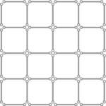
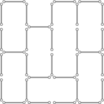
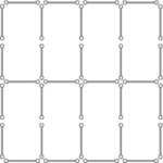
In matchsticks.pl, Boolean variables indicate whether a matchstick is placed at a specific position. The task is to eliminate all subsquares from the initial configuration in such a way that the maximum number of matchsticks is left in place:

We can use the CLP(B) predicate weighted_maximum/3 to show that we need to remove at least 9 matchsticks to eliminate all subsquares.

The left figure shows a sample solution, leaving the maximum number of matchsticks (31) in place. If you keep more matchsticks in place, subsquares remain. For example, the right figure contains exactly 7 subsquares, including the 4x4 outer square.

CLP(B) constraints can be used to quickly generate, test and count solutions of such puzzles, among many other applications. For example, there are precisely 62,382,215,032 subsquare-free configurations that use exactly 18 matchsticks. This is the maximum number of such configurations for any fixed number of matchsticks on this grid.

Independent sets and weighted kernels

As another example, consider the following graph:

It is the so-called cycle graph with 100 nodes, C₁₀₀. Using CLP(B) constraints, it is easy to see that this graph has exactly 792,070,839,848,372,253,127 independent sets, and exactly 1,630,580,875,002 maximal independent sets, which are also called kernels. The gray nodes in the next picture show one such kernel:

Suppose that we assign each node n_j the weight w_j = (-1)^νj, where νj denotes the number of ones in the binary representation of j. In the above figure, nodes with negative weight are drawn as squares, and nodes with positive weight are drawn as circles.

Only 5 nodes (1, 25, 41, 73 and 97) of this kernel with 38 nodes have negative weight in this case, for a total weight of 28. In this case, the example shows a kernel with maximum weight. It is easy to find such kernels with the CLP(B) predicate weighted_maximum/3, and we can also compute other interesting facts: For example, there are exactly 256 kernels of maximum weight in this case. There are exactly 25,446,195,000 kernels with exactly 38 nodes. All kernels have between 34 and 50 nodes. For any fixed number of nodes, the maximum number of kernels (492,957,660,000) is attained with 41 nodes, and among these kernels, the maximum total weight is 25.

By negating the coefficients of weighted_maximum/3, we can also find kernels with minimum weight. For example:

Implementation

The implementation of library(clpb) is based on ordered and reduced Binary Decision Diagrams (BDDs). BDDs are an important data structure for representing Boolean functions and have many virtues that often allow us to solve interesting tasks efficiently.

For example, the CLP(B) constraint sat(card([2],[X,Y,Z])) is translated to the following BDD:

To inspect the BDD representation of Boolean constraints, set the Prolog flag clpb_residuals to bdd. For example:

?- set_prolog_flag(clpb_residuals, bdd).
true.

?- sat(X+Y).
node(2)- (v(X, 0)->true;node(1)),
node(1)- (v(Y, 1)->true;false).

Using library(clpb) is a good way to learn more about BDDs. The variable order is determined by the order in which the variables are first encountered in constraints. You can enforce arbitrary variable orders by first posting a tautology such as +[1,V1,V2,...,Vn].

For example:

?- sat(+[1,Y,X]), sat(X+Y).
node(2)- (v(Y, 0)->true;node(1)),
node(1)- (v(X, 1)->true;false).

You can render CLP(B)'s residual goals as BDDs in SWISH using the BDD renderer.

ZDD-based variant of `library(clpb)`

There is a limited alternative version of library(clpb), based on Zero-suppressed Binary Decision Diagrams (ZDDs).

Please see the zdd directory for more information. Try the ZDD-based version for tasks where the BDD-based version runs out of memory. You must use zdd_set_vars/1 before using sat/1 though.

Acknowledgments

I am extremely grateful to:

Jan Wielemaker for providing the Prolog system that made all this possible in the first place.

Ulrich Neumerkel, who introduced me to constraint logic programming and CLP(B) in particular. If you are teaching Prolog, I strongly recommend you check out his GUPU system.

Nysret Musliu, my thesis advisor, whose interest in combinatorial tasks, constraint satisfaction and SAT solving highly motivated me to work in this area.

Mats Carlsson, the designer and main implementor of SICStus Prolog and its visionary CLP(B) library. For any serious use of Prolog and constraints, make sure to check out his elegant and fast system.

Donald Knuth for the superb treatment of BDDs and ZDDs in his books and programs.

triska/clpb