CLP(FD), Constraint Logic Programming over Finite Domains, is available in SWI-Prolog as library(clpfd).
This repository contains usage examples that illustrate important concepts and principles of the CLP(FD) library.
clpfd.pdf is a shortened version of the library documentation, intended as supplementary lecture material.
Read The Power of Prolog for more information, and in particular the introduction to declarative integer arithmetic.
See also the successor library, CLP(Z).
In the following, it is assumed that you have put the following
directive in your .swiplrc initialisation file:
:- use_module(library(clpfd)).
Putting this directive in your initialisation file is the recommended way to make integer constraints available in all your programs. This is advisable because almost all Prolog programs also reason about integers in one way or another.
Does an error like the following seem familiar to you?
?- 3 is 1+Y.
ERROR: is/2: Arguments are not sufficiently instantiated
CLP(FD) puts an end to such low-level limitations:
?- 3 #= 1+Y.
Y = 2.
When learning Prolog, use constraints to free your mind from procedural considerations, and focus on a declarative reading!
CLP(FD) is an instance of the general CLP(.) scheme, extending logic programming with reasoning over specialised domains.
In the case of CLP(FD), the domain is the set of integers.
CLP(FD) constraints like
(#=)/2,
(#\=)/2,
and
(#<)/2
are meant to be used as pure alternatives for lower-level arithmetic
primitives over integers. Importantly, they can be used in all
directions.
For example, we can use CLP(FD) constraints to obtain a version of
n_factorial/2 that can be used as a true relation:
n_factorial(0, 1).
n_factorial(N, F) :-
        N #> 0,
        N1 #= N - 1,
        F #= N * F1,
        n_factorial(N1, F1).
This works in all directions, for example:
?- n_factorial(47, F).
258623241511168180642964355153611979969197632389120000000000 ;
false.
and also:
?- n_factorial(N, 1).
N = 0 ;
N = 1 ;
false.
and also in the most general case:
?- n_factorial(N, F).
N = 0,
F = 1 ;
N = F, F = 1 ;
N = F, F = 2 ;
N = 3,
F = 6 .
This repository contains several example programs. The main predicates are all completely pure and can be used as true relations. This means that you can use the same program to:
- find a single solution
- enumerate all solutions
- complete partially instantiated solutions
- validate fully instantiated solutions.
To get an idea of the power, usefulness and scope of CLP(FD) constraints, I recommend you work through the examples in the following order:
-
n_factorial.pl: Shows how to use CLP(FD) constraints for declarative integer arithmetic, obtaining very general programs that can be used in all directions. Declarative integer arithmetic is the simplest and most common use of CLP(FD) constraints. They are easy to understand and use this way, and often increase generality and logical purity of your code.
-
sendmory.pl: A simple cryptoarithmetic puzzle. The task is to assign one of the digits 0,...,9 to each of the letters S,E,N,D,M,O,R and Y in such a way that the following calculation is valid, and no leading zeroes appear:
     S E N D
   + M O R E
   ---------
 = M O N E Y
This example illustrates several very important concepts:
-
It is the first example that shows residual constraints for the most general query. They are equivalent to the original query.
-
It is good practice to separate the core relation from
labeling/2, so that termination and determinism can be observed without an expensive search for concrete solutions. See the CLP(FD) documentation for more information about this subject. -
You can use this example to illustrate that the CLP(FD) system is able to propagate many things that can also be found with human reasoning. For example, due to the nature of the above calculation and the prohibition of leading zeroes,
Mis necessarily 1.
-
-
sudoku.pl: Uses CLP(FD) constraints to model and solve a simple and well-known puzzle. This example is well suited for understanding the impact of different propagation strengths: Use it to compare
all_different/1andall_distinct/1on different puzzles:The small dots in each cell indicate how many elements are pruned by different consistency techniques. In many Sudoku puzzles, using
all_distinct/1makes labeling unnecessary. Does this mean that we can forgetall_different/1entirely? -
magic_square.pl: CLP(FD) formulation of magic squares. This is a good example to learn about symmetry breaking constraints: Consider how you can eliminate solutions that are rotations, reflections etc. of other solutions, by imposing suitable further constraints. For example, the following two solutions are essentially identical, since one can be obtained from the other by reflecting elements along the main diagonal:
Can you impose additional constraints so that you get only a single solution in such cases, without losing any solutions that do not belong to the same equivalence class? How many solutions are there for N=4 that are unique up to isomorphism?
-
magic_hexagon.pl: Uses CLP(FD) to describe a magic hexagon of order 3. The task is to place the integers 1,...,19 in the following grid so that the sum of all numbers in a straight line (there are lines of length 3, 4 and 5) is equal to 38. One solution of this task is shown in the right picture:
This is an example of a task that looks very simple at first, yet is almost impossibly hard to solve manually. It is easy to solve with CLP(FD) constraints though. Use the constraint solver to show that the solution of this task is unique up to isomorphism.
-
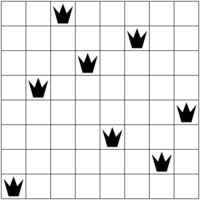
n_queens.pl: Model the so-called N-queens puzzle with CLP(FD) constraints. This example is a good candidate to experiment with different search strategies, specified as options of
labeling/2. For example, using the labeling strategyff, you can easliy find solutions for 100 queens and more. Sample solutions for 8 and 50 queens:Try to find solutions for larger N. Reorder the variables so that
ffbreaks ties by selecting more central variables first. -
knight_tour.pl: Closed Knight's Tour using CLP(FD) constraints. This is an example of using a more complex global constraint called
circuit/1. It shows how a problem can be transformed so that it can be expressed with a global constraint. Sample solutions, using an 8x8 and a 16x16 board:Decide whether
circuit/1can also be used to model tours that are not necessarily closed. If not, why not? If possible, do it. -
tasks.pl: A task scheduling example, using the
cumulative/2global constraint. Themin/1labeling option is used to minimize the total duration.
When studying Prolog and CLP(FD) constraints, it is often very useful to show animations of search processes. An instructional example:
N-queens animation: This visualizes the search process for the N-queens example.
You can use similar PostScript instructions to create custom animations for other examples.
Since integer arithmetic is in general undecidable, CLP(FD)
constraints are necessarily incomplete. This means that you cannot,
in general, take the fact that a CLP(FD) constraint succeeds as an
indication that there are any solutions. Therefore, you need to use
call_residue_vars/2
to see if any constraints are still pending. For example:
declarative_false :-
        X #< Y,
        Y #< X.
With the above program, we get:
?- declarative_false.
true.
however, it is in fact false, because there are no solutions! The
toplevel has omitted important constraints that are still pending. You
can make them visible by wrapping the goal in call_residue_vars/2:
?- call_residue_vars(declarative_false, Vs).
Vs = [X1, X2],
X1#=<X2+ -1,
X2#=<X1+ -1.
There is a solution only if you can satisfy these residual goals. Can you?
We have now seen several examples of CLP(FD) constraints being true relations that can be used in all directions.
Alas, some non-relational deficiencies still remain in the default
mode of library(clpfd). For example, consider the interaction:
?- X = 1+1, X #= 2.
X = 1+1.
and contrast it with exchanging the two goals:
?- X #= 2, X = 1+1.
false.
This difference is obvisouly undesirable: It breaks commutativity that we expect from logical conjunction. Even worse, this breaks monotonicity: By adding a further constraint, we obtain new solutions:
?- X = 1+1, X #= 2, X = 1+1.
X = 1+1.
How can such problematic cases even arise? The reason is that CLP(FD) expressions are defaulty: In CLP(FD) expressions, a logical variable is always regarded as standing for a concrete integer, although declaratively, it also stands for other CLP(FD) expressions that also make a given constraint true. For example, when we post the constraint:
?- X #= 2.
then we get the single solution X = 2. It is clear though that,
from a declarative point of view, X = 1+1, X = 0+2, X = 3-1+0
and other CLP(FD) expressions are also perfectly admissible
solutions. However, the constraint solver impurely commits to
treating each CLP(FD) variable as standing for a single integer.
The way to avoid defaultyness is, as always, to equip all entities with a dedicated functor. This way, the cases can be cleanly distinguished.
For this reason, library(clpfd) features a dedicated syntax to
mark variables that stand for concrete integers. This is
accomplished by wrapping them with #/1 (preferred)
or ?/1. For example:
?- #(X) #= 2.
X = 2.
If we consistently use this syntax in CLP(FD) constraints, then the discrepancy above cannot arise:
?- X = 1+1, #(X) #= 2.
ERROR: Type error: `integer' expected, found `1+1' (a compound)
and after exchanging the goals:
?- #(X) #= 2, X = 1+1.
false.
Note that a type error can be replaced by silent failure, so the two
cases are now really declaratively equivalent.
If you set the Prolog flag clpfd_monotonic to true, then CLP(FD)
is monotonic: In that mode, you get a clean instantiation error
if you use a variable without the #/1 wrapper in
CLP(FD) constraints.
For example:
?- set_prolog_flag(clpfd_monotonic, true).
true.

?- X #= 2.
ERROR: Arguments are not sufficiently instantiated

?- #(X) #= 2.
X = 2.
Set clpfd_monotonic to true to enjoy the utmost relational
benefits of CLP(FD).
Suppose for a moment that CLP(FD) constraints were not available in
your Prolog system, or that you do not want to use them. How do we
formulate n_factorial/2 with more primitive integer arithmetic?
In our first attempt, we simply replace the declarative CLP(FD) constraints by lower-level arithmetic predicates and obtain:
n_factorial(0, 1).
n_factorial(N, F) :-
        N > 0,
        N1 is N - 1,
        F is N * F1,
        n_factorial(N1, F1).
Unfortunately, this does not work at all, because lower-level arithmetic predicates are moded: This means that their arguments must be sufficiently instantiated at the time they are invoked. In fact, SWI-Prolog does not even compile the above code but yields an error at compilation time. Therefore, we must reorder the goals and — somewhat annoyingly — change this for example to:
n_factorial(0, 1).
n_factorial(N, F) :-
        N > 0,
        N1 is N - 1,
        n_factorial(N1, F1),
        F is N * F1.
Naive example queries inspired more by functional than by relational thinking may easily mislead us into believing that this version is working correctly:
?- n_factorial(6, F).
F = 720 ;
false.
Another example:
?- n_factorial(3, F).
F = 6 ;
false.
But what about more general queries? For example:
?- n_factorial(N, F).
N = 0,
F = 1 ;
ERROR: n_factorial/2: Arguments are not sufficiently instantiated
Unfortunately, this version thus cannot be directly used to enumerate more than one solution, which is another severe drawback in comparison with the pure version.
You can make the deficiency a lot worse by arbitrarily adding
a !/0 somewhere. Using !/0 is a quite reliable way to destroy
almost all declarative properties of your code in most cases, and this
example is no exception:
n_factorial(0, 1) :- !.
n_factorial(N, F) :-
        N > 0,
        N1 is N - 1,
        n_factorial(N1, F1),
        F is N * F1.
This version appears in several places. The fact that the following interaction incorrectly tells us that there is exactly one solution of the factorial relation is apparently no cause for concern there:
?- n_factorial(N, F).
N = 0,
F = 1.
Zero and one are the only important integers in any case, if you are mostly interested in programming at a very low level.
For more usable and general programs, I therefore recommend you stick to CLP(FD) constraints for integer arithmetic. You can place pure goals in any order without changing the declarative meaning of your program, just as you would expect from logical conjunction. For example:
n_factorial(0, 1).
n_factorial(N, F) :-
        N #> 0,
        N1 #= N - 1,
        n_factorial(N1, F1),
        F #= N * F1.
Reordering pure goals can change termination properties, but it cannot incorrectly lead to failure where there is in fact a solution. Therefore, we get with the above CLP(FD) version for example:
?- n_factorial(N, 3).
<loops>
And now we can reason completely declaratively about the code: Knowing that (a) CLP(FD) constraints are pure and can thus be reordered quite liberally and (b) that posting CLP(FD) constraints always terminates, we know that placing CLP(FD) constraints earlier can at most improve, never worsen the desirable termination properties.
Therefore, we change the definition to the version shown initially:
n_factorial(0, 1).
n_factorial(N, F) :-
        N #> 0,
        N1 #= N - 1,
        F #= N * F1,
        n_factorial(N1, F1).
The sample query now terminates:
?- n_factorial(N, 3).
false.
Using CLP(FD) constraints has allowed us to improve the termination properties of this predicate by purely declarative reasoning.
All current and future development of this library takes place as CLP(Z) for SICStus Prolog.
For ISO conformance, higher performance and professional support, it is strongly recommended that you obtain a copy of SICStus Prolog and use it for all serious Prolog development.
I am extremely grateful to:
Jan Wielemaker for providing the Prolog system that made all this possible in the first place.
Tom Schrijvers,
who has generously contributed several important constraint libraries
to SWI-Prolog
(dif/2!!),
and from whom I learned a lot.
Ulrich Neumerkel, who introduced me to constraint logic programming and was the first and most determined tester of my library, filing hundreds of comments. If you are teaching Prolog, I recommend you check out his GUPU system.
Nysret Musliu, my thesis advisor, whose interest in combinatorial tasks and constraint satisfaction highly motivated me to work in this area.
Mats Carlsson, the designer and main implementor of SICStus Prolog and its superb CLP(FD) library. For any serious use of CLP(FD) constraints, make sure to check out his elegant and fast system.


