Simulating particles and sedimentation in Glomma river

Langragian particle tracking framework Repository for developing sediment module for OpenDrift for modelling flow of particles in Glomma.

Code for animating particles and plotting trajectories have been added. Any plot or animation should be initialized using the config_plot.py file and the main script file create_maps_and_animations.py.

Run particle drift Run particle tracking of clay and sand particles of different diameters and densities after initializing config_sedimentdrift.py. The current setup initializes the diameters and densities of particles using aGaussian distribution function with mean and standard deviations as observed for Glomma in June 2020 using a LISST instrument.

self.diameters = self.generate_gaussian_distribution(0.05e-3, 0.01e-3/3., self.number_of_particles)
self.densities = self.generate_gaussian_distribution(1200, 1000/3., self.number_of_particles)

Calculate sedimentation After running the model we now have to analyse the output. This is done using various plotting and animation scripts (see below) but the key script is called probability_distibution_v2.py. The script organizes the simulation results by grouping into individual trajectories.

df = xr.open_mfdataset(file_list, concat_dim='trajectory', combine='nested')
ds = df.groupby(df.trajectory).apply(self.extract_data, args=(filter_options,))

Once grouped we can filter the data per trajectory to only analyse what we are interested in. This is done by submitting an options dictionary to the groupby.apply function.

 filter_options = {"density_min": 0,
                   "density_max": 2000.,
                   "selected_month": 2,
                   "selected_day": 7,
                   "status": 1}

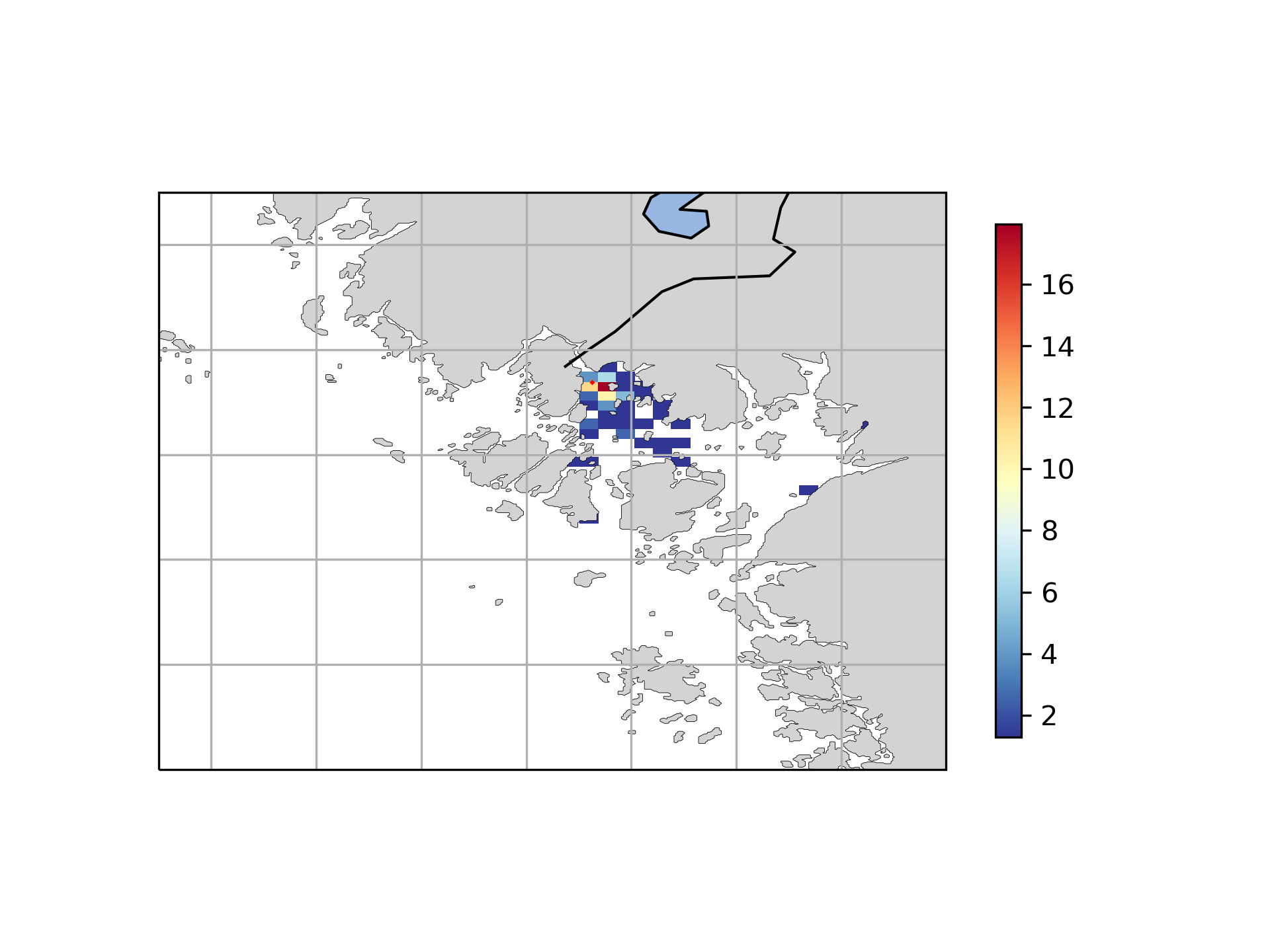
This particular filter will keep only particles with densities between 0 to 2000, for month 2 (February), day 7, and only keep particles that have settled on the bottom (status=1). The data are then organized into bins that cover the region of interest with the given resolution of interest. For example, you can define the resolution of the bins to be 1km, 1m or whatever you want and this is done in the file config_plot.py. The histogram is then calculated for the bins and displayed as a pcolormesh plot.

Notes on filtering approach The resulting datafiles after running Opendrift can contain millions of locations for thousands of particles. To quickly filter the results to just work with the data we are interested in, e.g. the location where particles settled, we apply a few tricks to speed things up. First of all, after reading the datafiles using xarray we convert the datasets to pandas dataframes. Next we convert the dataframe to a dask.dataframe which allows us to utilize Dask to filter the data using paralell processing. After the filtering has finished, the result is a Pandas dataframe which we run groupby("trajectory") and finally convert back to a xarray.Dataarray.

        # Get the data and group by trajectory
        df = xr.open_mfdataset(file_list, concat_dim='trajectory', combine='nested').to_dataframe()
        # Convert from multi-index (date - trajectory) to single index (date) to use Dask
        df = df.reset_index(level="time")

        # Convert to Dask dataframe with chunks
        ddf = dd.from_pandas(df, 10)

        # This one returns a Pandas dataframe
        ddf = self.filter_data(ddf, filter_options).compute()

        ddf = ddf.set_index(['time', ddf.index])
        ds = ddf.groupby("trajectory").apply(self.return_ds).to_xarray()

Plotting

create_maps_and_animations.py - main plot script
config_plot.py - configure and setup common plot properties
animate_catter.py - class for animating particles
particle_tracks.py - class for plotting the particle trajectories
plot_particles_at_depth.py- plots time versus depth for three different densities / density ranges of clay

unittests A number of simple unittests are used to ensure that the methods of the toolbox behaves as they should once changes have been pushed to Github. The tests are all unittests but we use nose2to run the tests and to collect coverage information.

nose2 --with-coverage

16.07.2020 - updated unit tests to include tests for generating diameter, densities, and calculating terminal velocity for various buoyancies.

trondkr/Glomma_particles

Simulating particles and sedimentation in Glomma river