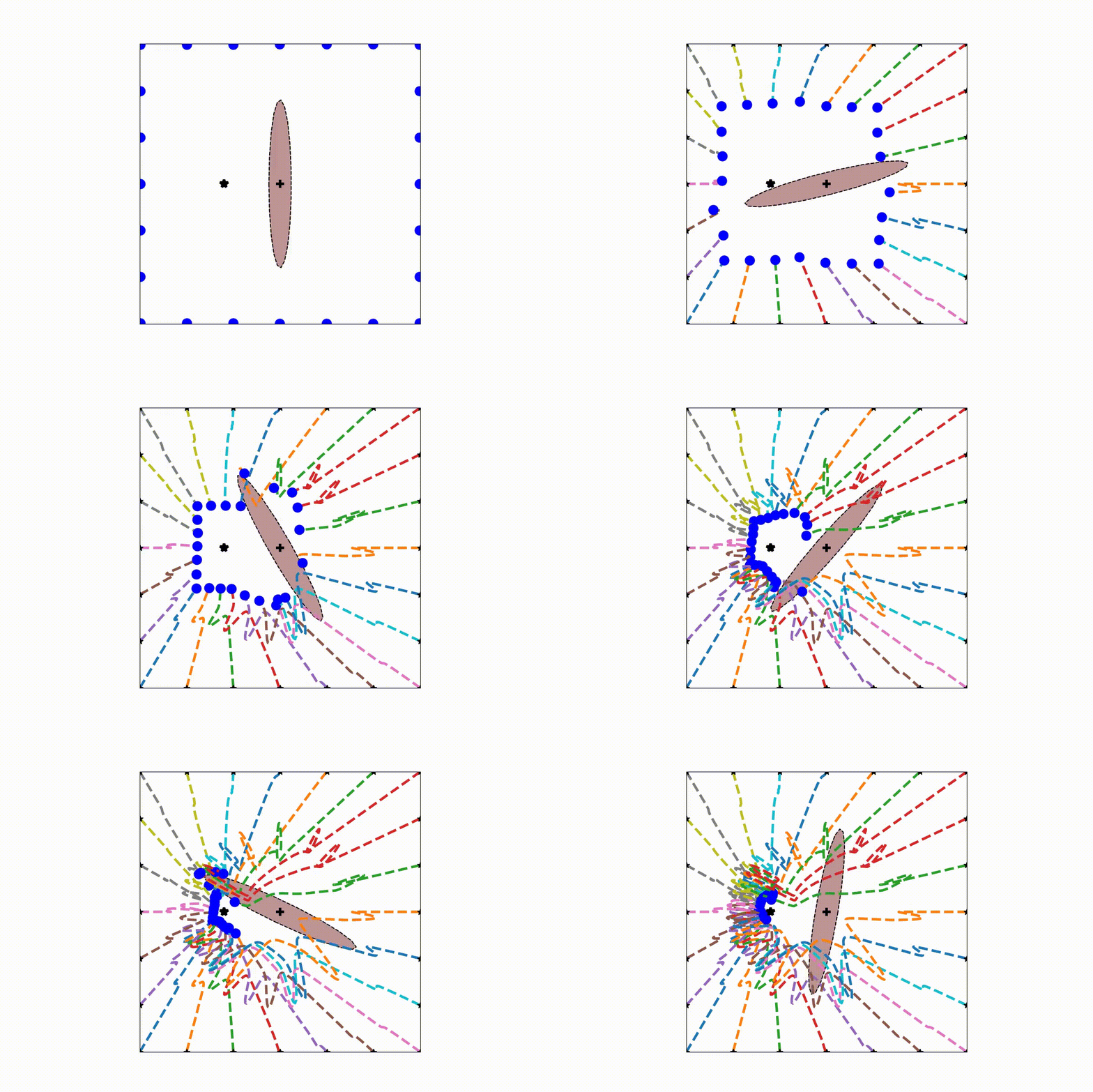
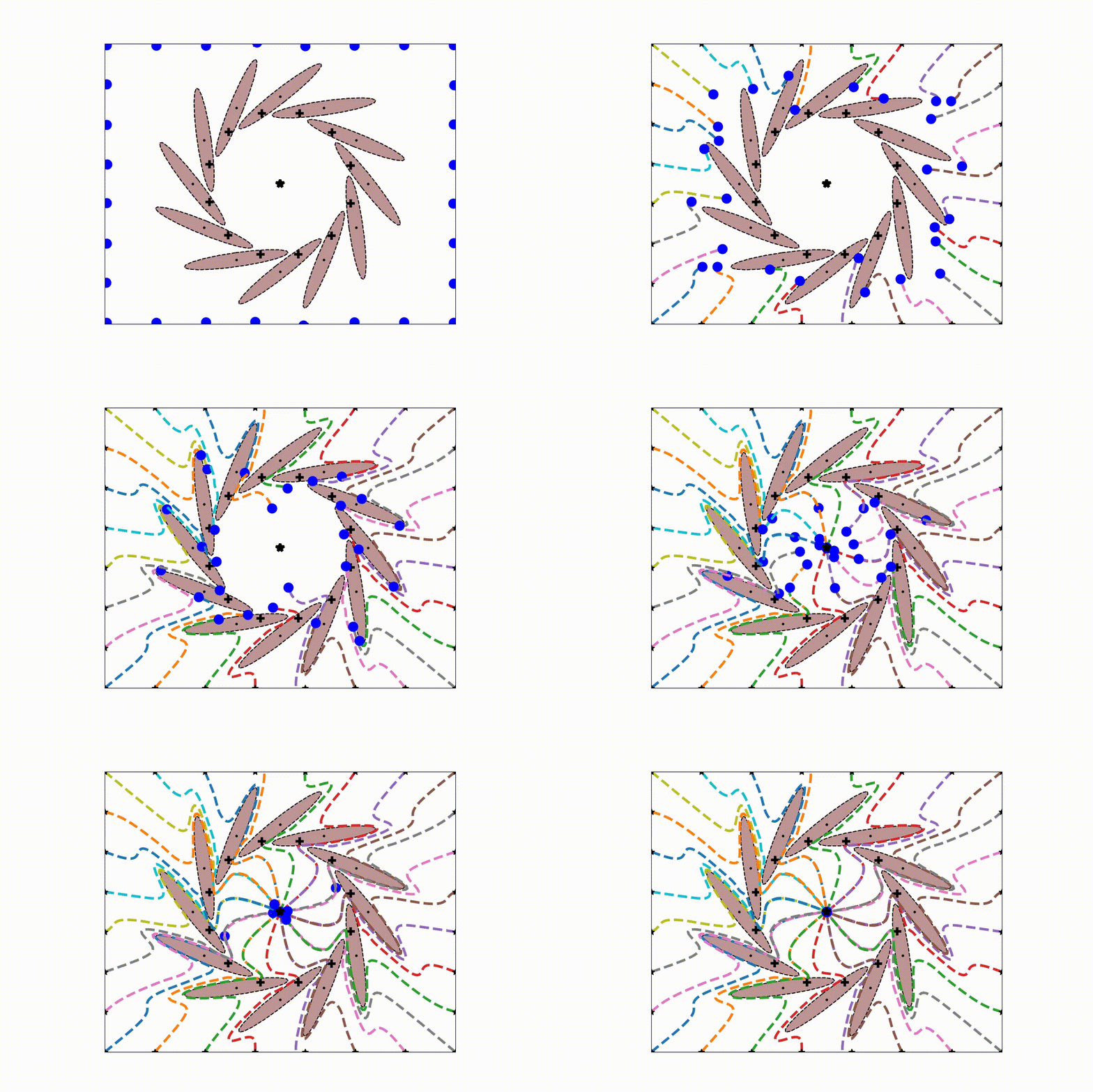
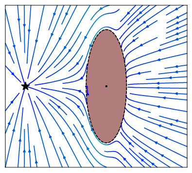
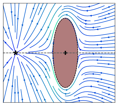
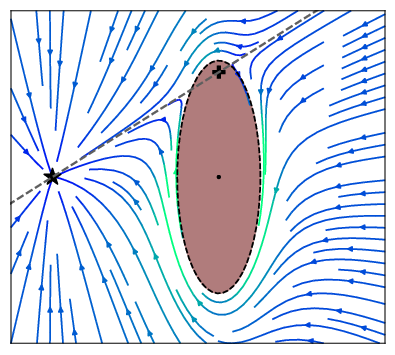
This package contains a dynamic obstacle avoidance algorithm for concave and convex obstacles as developped in [1]. The algorithm is an extension of the work of [2].
Requirements: conda, jupyter notebook, python.
To setup got to your install/code directory, and type:
git clone https://github.com/epfl-lasa/dynamic_obstacle_avoidance_linear
conda env create -f environment.yml
conda activate obstacle_avoidance_linear
python setup.py install
There is an interactive jupyter module, to familarize with the algorithm. From the install/code directory it can by run with:
cd notebook
jupyter notebook
To execute an interactive script online click here:
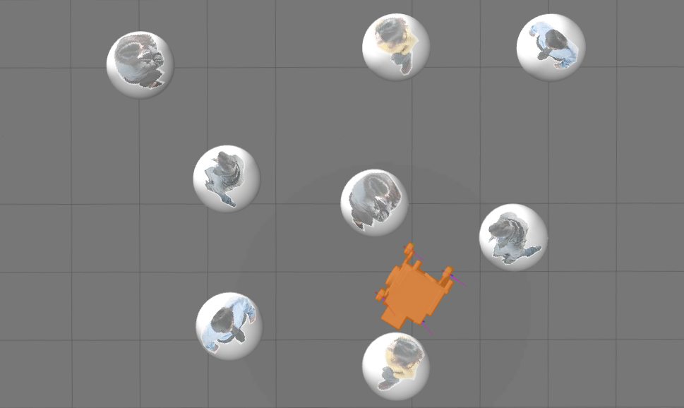
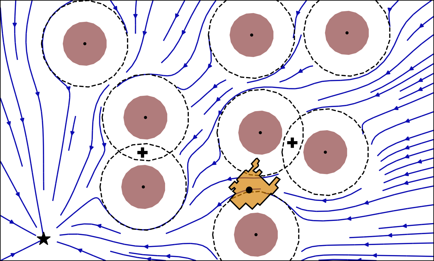
Several examples of the obstacle avoidance algorithm have been ipmlemented. The highly reactive nature of the algorithm allows it to be used to avoid crowded environment with fastly chaning movement of humans.
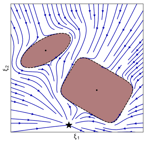
Different examples of the vector field simulation can be launched by running the script
examples_vectorField.py
The simulation number can be specified to run each specific simulation. The resolution indicates the number of grid points along each axis. Further more figures can be saved automatically into the <> folder.
Custom vector fields can be created using by calling the class
Simulation_vectorFields() [$ lib_visalization/vectorField_visualization.py]
Different animated examples with static and non-static obstacles can be found in:
examples_animation.py
The simulation number can be specified to choose between the animations. Further it can be saved directly to a MP4 video.
Custom vector animation can be created by running the function
run_animation() [$ lib_visalization/animated_simulation.py]
For each obstacle of an ellipsoid form, a class instanse of "lib_obstacleAvoidance/obstacle_class.py" has to be defined. This desires several paramters such as center position x0, axis length a, surface curvature p, orientation th_r. Moving obstacles additionally have a linear velocity xd and an angular velocity w.
For the modulation towards a general obstacle needs a reference point within the obstacle, the distance to the obstacle and the tangent hyperplane.
An ellipsoid obstacle can be created using the class
class_obstacle() [$ lib_obstacleAvoidance/class_obstacle.py]
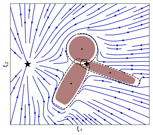
An initial (linear) dynamical system is modulated around obstacles. The modulation works in real-time and dynamically around any number of obstacles. Convergence towards an attractor can be ensured, as long as intersecting obstacles can be described with a star shape. Detailled information can be found in [1]. The modulation is performed with the function
obs_avoidance_interpolation_moving() in [$ lib_obstacleAvoidance/linear_modulations.py]
It takes as argument the position x of the modulation, the initial dynamial system xd and a list of obstacles obs. Optional arguments are the position and the hyperparameter weightPow, which defines the weighting function.
A RK4 integration uses the function:
obs_avoidance_rk4() in [$ lib_obstacleAvoidance/linear_modulations.py]
Helping functions are defined in the "lib_obstacleAvoidance/linear_modulations.py".
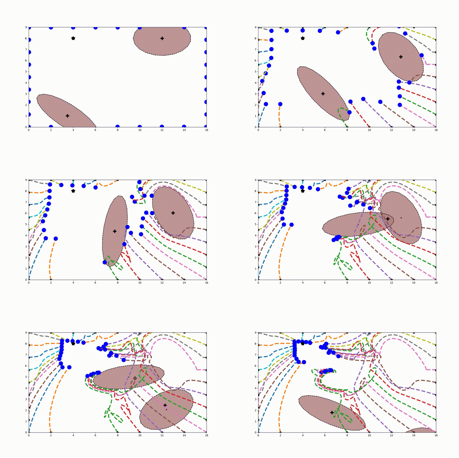
At the heart of the present obstacle avoidance algorithm lies the correct placement of the reference point within the obstacle. It ensures convergence towards the attractor and defines the split of the DS.
Automatic and dynamic placement of the reference point is done with the functions of the dynamic center are applied with "lib_obstacleAvoidance/obs_common_section.py" and "lib_obstacleAvoidance/obs_dynamic_center_3d.py".
 </>
</>
Complexer obstacles can either be formed using several ellipses, which already allows to form many star shaped obstacles. Note, more complex obstacles can be formed with an analytical description of the surface of the obstacle, but this module can not handle it yet
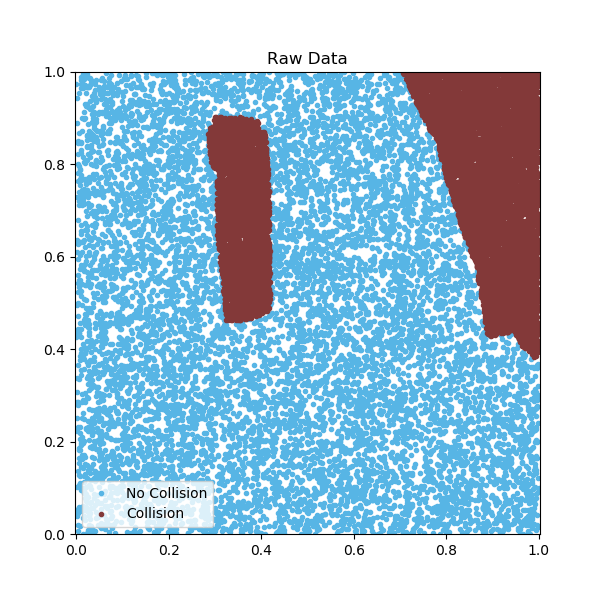
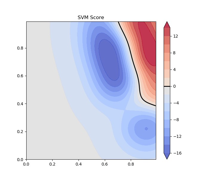
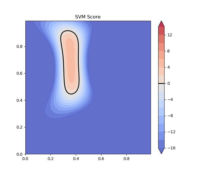
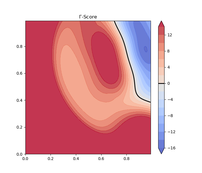
Obstacles can be learned using SVM (or other regression methods). This way a svm-function can be learned for each obstacles. See for the case of 2D data bellow:
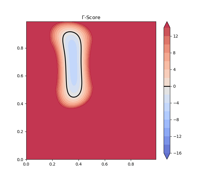
From this SVM score a Gamma-function can be established which is used for the calculation of the modulation matrix (including the derived normal):
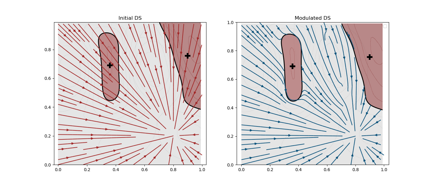
This allows then to modulate the system and guide a (in this case linear) dynamical system around a learned environment of obstacles:
This pictures can be recreated by running the file scripts/test_learning_obstacle_gradient.py. A new 'learning' obstacle should be created similar to the LearningObstacle-class found in the file ObstacleAvoidance/obstacle_learning.py.
References
[1] Huber, Lukas, Aude Billard, and Jean-Jacques E. Slotine. "Avoidance of Convex and Concave Obstacles with Convergence ensured through Contraction." IEEE Robotics and Automation Letters (2019).
[2] Khansari-Zadeh, Seyed Mohammad, and Aude Billard. "A dynamical system approach to realtime obstacle avoidance." Autonomous Robots 32.4 (2012): 433-454.
Contact: [Lukas Huber] (http://lasa.epfl.ch/people/member.php?SCIPER=274454) (lukas.huber AT epfl dot ch)
Acknowledgments This work was funded in part by the EU project Crowdbots.
