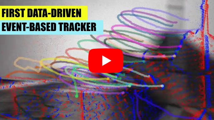
Data-driven Feature Tracking for Event Cameras

This is the code for the CVPR23 paper Data-driven Feature Tracking for Event Cameras (PDF) by Nico Messikommer*, Carter Fang*, Mathis Gehrig, and Davide Scaramuzza. For an overview of our method, check out our video.

If you use any of this code, please cite the following publication:

@Article{Messikommer23cvpr,
  author  = {Nico Messikommer* and Carter Fang* and Mathias Gehrig and Davide Scaramuzza},
  title   = {Data-driven Feature Tracking for Event Cameras},
  journal = {IEEE Conference on Computer Vision and Pattern Recognition},
  year    = {2023},
}

Abstract

Because of their high temporal resolution, increased resilience to motion blur, and very sparse output, event cameras have been shown to be ideal for low-latency and low-bandwidth feature tracking, even in challenging scenarios. Existing feature tracking methods for event cameras are either handcrafted or derived from first principles but require extensive parameter tuning, are sensitive to noise, and do not generalize to different scenarios due to unmodeled effects. To tackle these deficiencies, we introduce the first data-driven feature tracker for event cameras, which leverages low-latency events to track features detected in a grayscale frame. We achieve robust performance via a novel frame attention module, which shares information across feature tracks. By directly transferring zero-shot from synthetic to real data, our data-driven tracker outperforms existing approaches in relative feature age by up to 120% while also achieving the lowest latency. This performance gap is further increased to 130% by adapting our tracker to real data with a novel self-supervision strategy.

Content

This document describes the usage and installation for this repository.

Installation
Test Sequences and Pretrained Weights
Preparing Synthetic Data
Training on Synthetic Data
Preparing Pose Data
Training on Pose Data
Preparing Evaluation Data
Running Ours
Evaluation
Visualization

Installation

This guide assumes use of Python 3.9.7

If desired, a conda environment can be created using the following command:

conda create -n <env_name>

Install the dependencies via the requirements.txt file
pip install -r requirements.txt

Dependencies for training:
- PyTorch
- Torch Lightning
- Hydra
Dependencies for pre-processing:
- numpy
- OpenCV
- H5Py and HDF5Plugin
Dependencies for visualization:
- matplotlib
- seaborn
- imageio

Test Sequences and Pretrained Weights

To facilitate the evaluation of the tracking performance, we provide the raw events, multiple event representation, etc., for the used test sequences of the Event Camera Dataset and the EDS dataset. The ground truth tracks for both EC and EDS datasets generated based on the camera poses and KLT tracks can be downloaded here.

Furthermore, we also provide the network weights trained on the Multiflow dataset, the weights fine-tuned on the EC, and fine-tuned on the EDS dataset using our proposed pose supervision strategy.

Preparing Synthetic Data

Download MultiFlow Dataset

Download links:

If you use this dataset in an academic context, please cite:

@misc{Gehrig2022arxiv,
 author = {Gehrig, Mathias and Muglikar, Manasi and Scaramuzza, Davide},
 title = {Dense Continuous-Time Optical Flow from Events and Frames},
 url = {https://arxiv.org/abs/2203.13674},
 publisher = {arXiv},
 year = {2022}
}

The models were pre-trained using an older version of this dataset, available at the time of the submission. The download links above link to the up-to-date version of the dataset.

Pre-Processing Instructions

Preparation of the synthetic data involves generating input representations for the Multiflow sequences and extracting the ground-truth tracks.

To generate ground-truth tracks, run:
python data_preparation/synthetic/generate_tracks.py <path_to_multiflow_dataset> <path_to_multiflow_extras_dir>

Where the Multiflow Extras directory contains data needed to train our network such as the ground-truth tracks and input event representations.

To generate input event representations, run:
python data_preparation/synthetic/generate_event_representations <path_to_multiflow_dataset> <path_to_multiflow_extras_dir> <representation_type>

The resulting directory structure is:

multiflow_reloaded_extra/
├─ sequence_xyz/
│  ├─ events/
│  │  ├─ 0.0100/
│  │  │  ├─ representation_abc/
│  │  │  │  ├─ 0400000.h5
│  │  │  │  ├─ 0410000.h5
│  │  ├─ 0.0200/
│  │  │  ├─ representation_abc/
│  │
│  ├─ tracks/
│  │  ├─ shitomasi.gt.txt

Training on Synthetic Data

Training on synthetic data involves configuring the dataset, model, and training. The high-level config is at configs/train_defaults.yaml.

To configure the dataset:

Set data field to mf
Configure the synthetic dataset in configs/data/mf.yaml
Set the track_name field (default is shitomasi_custom)
Set the event representation (default is SBT Max, referred to as time_surfaces_v2_5 here)

Important parameters in mf.yaml are:

augment - Whether to augment the tracks or not. The actual limits for augmentations are defined as global variables in utils/datasets.py
mixed_dt - Whether to use both timesteps of 0.01 and 0.02 during training.
n_tracks/val - Number of tracks to use for validation and training. All tracks are loaded, shuffled, then trimmed.

To configure the model, set the model field to one of the available options in configs/model. Our default model is correlation3_unscaled.

To configure the training process:

Set the learning rate in configs/optim/adam.yaml (Default is 1e-4)
In configs/training/supervised_train.yaml, set the sequence length schedule via init_unrolls, max_unrolls, unroll_factor, and the schedule. At each of the specified training steps, the number of unrolls will be multiplied by the unroll factor.
Configure the synthetic dataset in configs/data/mf.yaml

The last parameter to set is experiment for organizational purposes.

With everything configured, we can begin training by running

CUDA_VISIBLE_DEVICES=<gpu_id> python train.py

Hydra will then instantiate the dataloader and model. PyTorch Lightning will handle the training and validation loops. All outputs (checkpoints, gifs, etc) will be written to the log directory.

The correlation_unscaled model inherits from models/template.py since it contains the core logic for training and validation. At each training step, event patches are fetched for each feature track (via TrackData instances) and concatenated prior to inference. Following inference, the TrackData instances accumulate the predicted feature displacements. The template file also contains the validation logic for visualization and metric computation.

To inspect models during training, we can launch an instance of tensorboard for the log directory: tensorboard --logdir <log_dir>.

Preparing Pose Data

To prepare pose data for fine-tuning, we need to rectify the data, run colmap, and generate event representations.

To rectify the data, run python data_preparation/real/rectify_ec.py or python data_preparation/real/eds_rectify_events_and_frames.py.

To refine the pose data with colmap, see data_preparation/colmap.py. We first run colmap.py generate. This will convert the pose data to a readable format for COLMAP to serve as an initial guess, generated in the colmap directory of the sequence. We then follow the instructions here from the COLMAP FAQ regarding refining poses.

Essentially:

Navigate to the colmap directory of a sequence
colmap feature_extractor --database_path database.db
colmap exhaustive_matcher --database_path database.db --image_path ../images_corrected
colmap point_triangulator --database_path database.db --image_path ../images_corrected/ --input_path . --output_path .
Launch the colmap gui, import the model files, and re-run Bundle Adjustment ensuring that only extrinsics are refined.
Run colmap.py extract to convert the pose data from COLMAP format back to our standard format.

To generate event representations, run python data_preparation/real/prepare_eds_pose_supervision.py or prepare_ec_pose_supervision.py. These scripts generate r event representations between frames. The time-window of the last event representation in the interval is trimmed. Currently, these scripts only support SBT-Max as a representation.

Training on Pose Data

To train on pose data, we again need to configure the dataset, model, and training. The model configuration is the same as before. The data field now needs to be set to pose_ec, and configs/data/pose_ec.yaml must be configured.

Important parameters to set in pose.yaml include:

root_dir - Directory with prepared pose data sequences.
n_frames_skip - How many frames to skip when chunking a sequence into several sub-sequences for pose training.
n_event_representations_per_frame - r value used when generating the event representations.

In terms of dataset configuration must also set pose_mode = True in utils/dataset.py. This overrides the loading of event representations from the time-step directories (eg 0.001) and instead from the pose data directories (eg pose_3).

In terms of the training process, for pose supervision we use a single sequence length so init_unrolls and max_unrolls should be the same value. Also, the schedule should have a single value indicating when to stop training. The default learning rate for pose supervision is 1e-6.

Since we are fine-tuning on pose, we must also set the checkpoint_path in configs/training/pose_finetuning_train_ec.yaml to the path of our pretrained model.

We are then ready to run train.py and fine-tune the network. Again, during training, we can launch tensorboard. For pose supervision, the re-projected features are visualized.

Running Ours

Preparing Input Data

The SequenceDataset class is responsible for loading data for inference. It expects a similar data format for the sequence as with synthetic training:

sequence_xyz/
├─ events/
│  ├─ 0.0100/
│  │  ├─ representation_abc/
│  │  │  ├─ 0000000.h5
│  │  │  ├─ 0010000.h5
├─ images_corrected/

To prepare a single sequence for inference, we rectify the sequence, a sequence segment, and generate event representations.

Rectification

For the EDS dataset, we download the txt-based version of a sequence and run data_preparation/real/eds_rectify_events_and_frames.py.
For the Event-Camera dataset, we download the txt-based version of a sequence and run data_preparation/real/rectify_ec.py.

Sequence Cropping and Event Generation

For the EDS dataset, we run data_preparation/real/prepare_eds_subseq with the index range for the cropped sequence as inputs. This will generate a new sub-sequence directory, copy the relevant frames for the selected indices, and generate event representations.

Inference

The inference script is evaluate_real.py and the configuration file is eval_real_defaults.yaml. We must set the event representation and checkpoint path before running the script.

The list of sequences is defined in the EVAL_DATASETS variable in evaluate_real.py. The script iterates over these sequences, instantiates a SequenceDataset instance for each one, and performs inference on the event representations generated in the previous section.

For benchmarking, the provided feature points need to be downloaded and used in order to ensure that all methods use the same features. The gt_path needs to be set in eval_real_defaults.yaml to the directory containing the text files.

Evaluation

Once we have predicted tracks for a sequence using all methods, we can benchmark their performance using scripts/benchmark.py. This script loads the predicted tracks for each method and compares them against the re-projected, frame-based ground-truth tracks, which can be downloaded here.
Inside the scripts/benchmark.py, the evaluation sequences, the results directory, the output directory and the name of the test methods <method_name_x> need to be specified. The result directory should have the following structure:

sequence_xyz/
├─ gt/
│  ├─ <seq_0>.gt.txt
│  ├─ <seq_1>.gt.txt
│  ├─ ...
├─ <method_name_1>/
│  ├─ <seq_0>.txt
│  ├─ <seq_1>.txt
│  ├─ ...
├─ <method_name_2>/
│  ├─ <seq_0>.txt
│  ├─ <seq_1>.txt
│  ├─ ...

The results are printed to the console and written to a CSV in the output directory.

uzh-rpg/deep_ev_tracker