FlowNetPytorch

Pytorch implementation of FlowNet by Dosovitskiy et al.

This repository is a torch implementation of FlowNet, by Alexey Dosovitskiy et al. in PyTorch. See Torch implementation here

This code is mainly inspired from official imagenet example. It has not been tested for multiple GPU, but it should work just as in original code.

The code provides a training example, using the flying chair dataset , with data augmentation. An implementation for Scene Flow Datasets may be added in the future.

Two neural network models are currently provided, along with their batch norm variation (experimental) :

FlowNetS
FlowNetSBN
FlowNetC
FlowNetCBN

Pretrained Models

Thanks to Kaixhin you can download a pretrained version of FlowNetS (from caffe, not from pytorch) here. This folder also contains trained networks from scratch.

Note on networks loading

Directly feed the downloaded Network to the script, you don't need to uncompress it even if your desktop environment tells you so.

Note on networks from caffe

These networks expect a BGR input (compared to RGB in pytorch). However, BGR order is not very important.

Prerequisite

these modules can be installed with pip

pytorch >= 1.2
tensorboard-pytorch
tensorboardX >= 1.4
spatial-correlation-sampler>=0.2.1
imageio
argparse
path.py

pip install -r requirements.txt

Training on Flying Chair Dataset

First, you need to download the the flying chair dataset . It is ~64GB big and we recommend you put it in a SSD Drive.

Default HyperParameters provided in main.py are the same as in the caffe training scripts.

Example usage for FlowNetS :

python main.py /path/to/flying_chairs/ -b8 -j8 -a flownets

We recommend you set j (number of data threads) to high if you use DataAugmentation as to avoid data loading to slow the training.

For further help you can type

python main.py -h

Visualizing training

Tensorboard-pytorch is used for logging. To visualize result, simply type

tensorboard --logdir=/path/to/checkoints

Training results

Models can be downloaded here in the pytorch folder.

Models were trained with default options unless specified. Color warping was not used.

Arch	learning rate	batch size	epoch size	filename	validation EPE
FlowNetS	1e-4	8	2700	flownets_EPE1.951.pth.tar	1.951
FlowNetS BN	1e-3	32	695	flownets_bn_EPE2.459.pth.tar	2.459
FlowNetC	1e-4	8	2700	flownetc_EPE1.766.pth.tar	1.766

Note : FlowNetS BN took longer to train and got worse results. It is strongly advised not to you use it for Flying Chairs dataset.

Validation samples

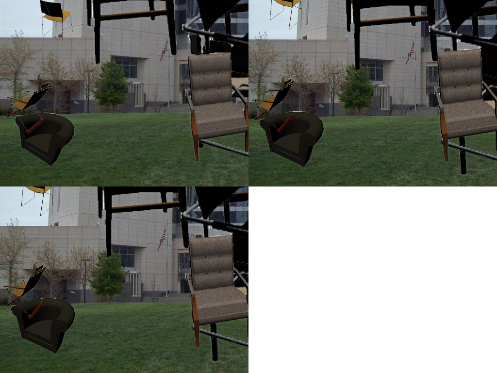
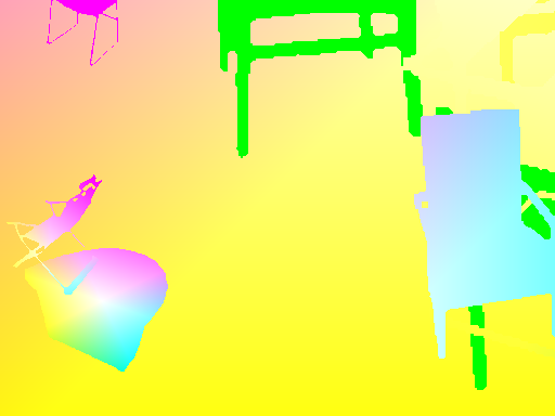
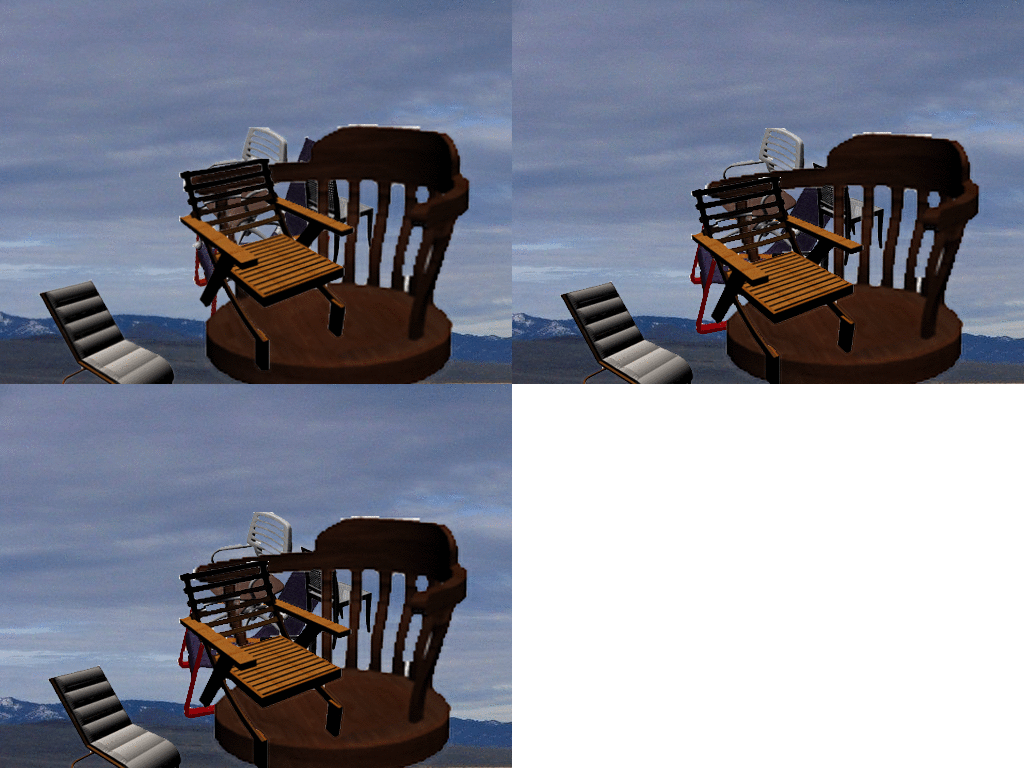
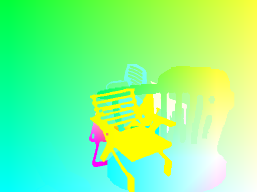
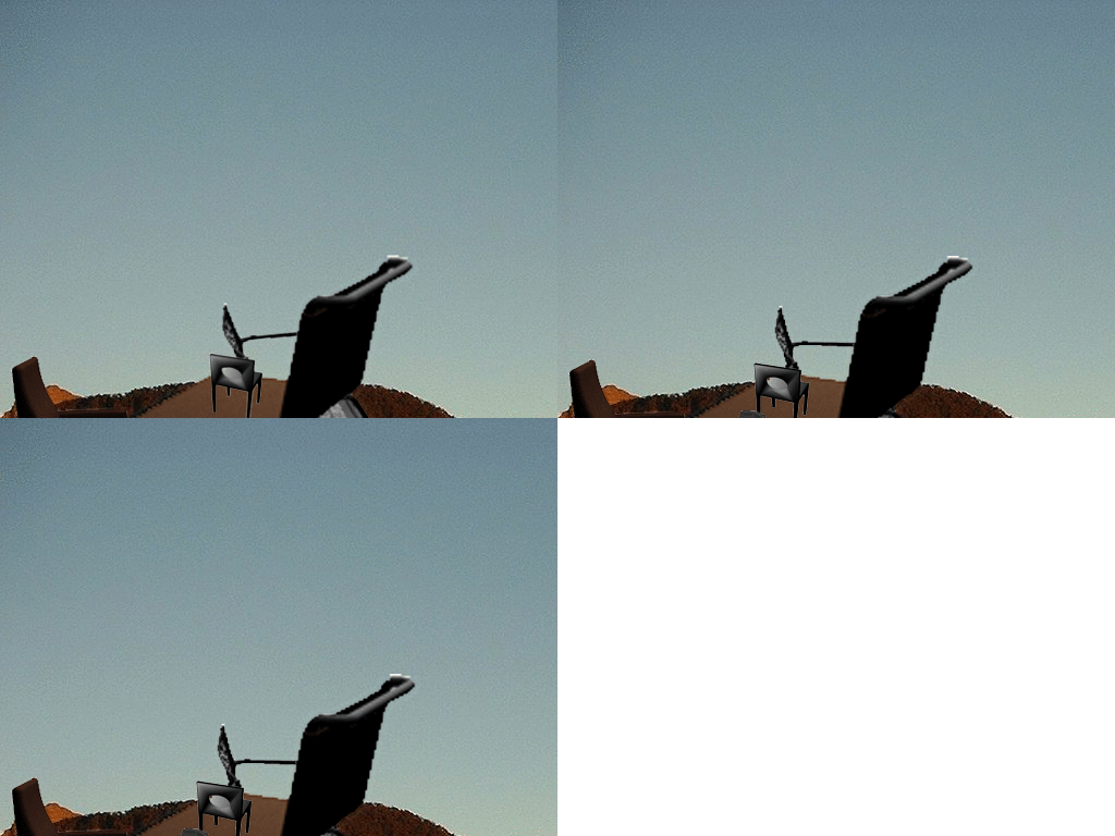
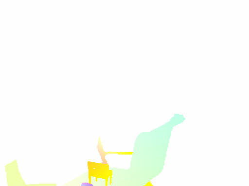
Prediction are made by FlowNetS.

Exact code for Optical Flow -> Color map can be found here

Input	prediction	GroundTruth

Running inference on a set of image pairs

If you need to run the network on your images, you can download a pretrained network here and launch the inference script on your folder of image pairs.

Your folder needs to have all the images pairs in the same location, with the name pattern

{image_name}1.{ext}
{image_name}2.{ext}

python3 run_inference.py /path/to/images/folder /path/to/pretrained

As for the main.py script, a help menu is available for additional options.

Note on transform functions

In order to have coherent transformations between inputs and target, we must define new transformations that take both input and target, as a new random variable is defined each time a random transformation is called.

Flow Transformations

To allow data augmentation, we have considered rotation and translations for inputs and their result on target flow Map. Here is a set of things to take care of in order to achieve a proper data augmentation

The Flow Map is directly linked to img1

If you apply a transformation on img1, you have to apply the very same to Flow Map, to get coherent origin points for flow.

Translation between img1 and img2

Given a translation (tx,ty) applied on img2, we will have

flow[:,:,0] += tx
flow[:,:,1] += ty

Scale

A scale applied on both img1 and img2 with a zoom parameters alpha multiplies the flow by the same amount

flow *= alpha

Rotation applied on both images

A rotation applied on both images by an angle theta also rotates flow vectors (flow[i,j]) by the same angle

\for_all i,j flow[i,j] = rotate(flow[i,j], theta)

rotate: x,y,theta ->  (x*cos(theta)-x*sin(theta), y*cos(theta), x*sin(theta))

Rotation applied on img2

Let us consider a rotation by the angle theta from the image center.

We must tranform each flow vector based on the coordinates where it lands. On each coordinate (i, j), we have:

flow[i, j, 0] += (cos(theta) - 1) * (j  - w/2 + flow[i, j, 0]) +    sin(theta)    * (i - h/2 + flow[i, j, 1])
flow[i, j, 1] +=   -sin(theta)    * (j  - w/2 + flow[i, j, 0]) + (cos(theta) - 1) * (i - h/2 + flow[i, j, 1])

vrmn/FlowNetPytorch