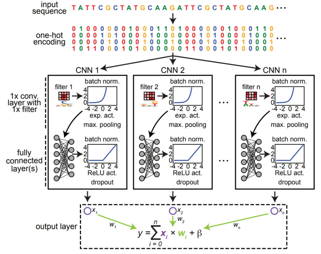
ExplaiNN is an adaptation of neural additive models (NAMs) for genomic tasks, where predictions are computed as a linear combination of multiple independent CNNs. Each CNN consists of a single convolutional filter and fully connected layers. This approach combines the expressivity of CNNs with the interpretability of linear models, providing global (cell state level) as well as local (individual sequence level) insights into the studied biological processes.
ExplaiNN requires Python 3.x with the following dependencies:
Additionally, the parsers, trainers, interpreters, etc. provided in the ./scripts folder require:
Biopythonclickandclick_option_groupfastclusterlogomakerpybedtoolsSciPyscikit-learn- The
MEMEsuite
git clone https://github.com/wassermanlab/ExplaiNN.git
cd ExplaiNN
python setup.py install
A normal successful installation should finish in a few minutes.
Below is an example of how to train and interpret an ExplaiNN model for predicting the binding of the TFs FOXA1, MAX, and JUND. The dataset can be found here.
Imports:
from matplotlib import pyplot as plt
import numpy as np
import os
import pandas as pd
import seaborn as sns
from sklearn.metrics import average_precision_score
from sklearn import metrics
import torch
from torch import nn

from explainn import tools
from explainn import networks
from explainn import train
from explainn import test
from explainn import interpretation
Model and parameter initialization:
device = torch.device("cuda:0" if torch.cuda.is_available() else "cpu")

# Hyper parameters
num_epochs = 15
batch_size = 128
learning_rate = 0.001

h5_file = "./data/test/tf_peaks_TEST_sparse_Remap.h5"
if not os.path.exists(h5_file):
    os.system(f"zless {h5_file}.gz > {h5_file}")

dataloaders, target_labels, train_out = tools.load_datas(h5_file,
                                                         batch_size,
                                                         0,
                                                         True)

target_labels = [i.decode("utf-8") for i in target_labels]

num_cnns = 100
input_length = 200
num_classes = len(target_labels)
filter_size = 19


model = networks.ExplaiNN(num_cnns, input_length, num_classes, filter_size).to(device)

criterion = nn.BCEWithLogitsLoss()
optimizer = torch.optim.Adam(model.parameters(), lr=learning_rate)Code for training the model
weights_folder = "./data/test/weights"
if not os.path.exists(weights_folder):
    os.makedirs(weights_folder)

model, train_error, test_error = train.train_explainn(dataloaders["train"],
                                                      dataloaders["valid"],
                                                      model,
                                                      device,
                                                      criterion,
                                                      optimizer,
                                                      num_epochs,
                                                      weights_folder,
                                                      name_ind="",
                                                      verbose=True,
                                                      trim_weights=False,
                                                      checkpoint=0,
                                                      patience=0)

tools.showPlot(train_error, test_error, "Loss trend", "Loss")
Epoch [1], Current Train Loss: 0.59987, Current Val Loss: 0.56369
Epoch [2], Current Train Loss: 0.54444, Current Val Loss: 0.53805
Epoch [3], Current Train Loss: 0.52748, Current Val Loss: 0.53336
Epoch [4], Current Train Loss: 0.51762, Current Val Loss: 0.53094
Epoch [5], Current Train Loss: 0.50993, Current Val Loss: 0.53307
Epoch [6], Current Train Loss: 0.50374, Current Val Loss: 0.53503
Epoch [7], Current Train Loss: 0.49772, Current Val Loss: 0.53951
Epoch [8], Current Train Loss: 0.49197, Current Val Loss: 0.54223
Epoch [9], Current Train Loss: 0.48682, Current Val Loss: 0.54598
Epoch [10], Current Train Loss: 0.48281, Current Val Loss: 0.54929
...model.load_state_dict(torch.load(f"{weights_folder}/{os.listdir(weights_folder)[0]}"))
labels_E, outputs_E = test.run_test(model, dataloaders["test"], device)
pr_rec = average_precision_score(labels_E, outputs_E)
no_skill_probs = [0 for _ in range(len(labels_E[:, 0]))]
ns_fpr, ns_tpr, _ = metrics.roc_curve(labels_E[:, 0], no_skill_probs)
roc_aucs = {}
raw_aucs = {}
roc_prcs = {}
raw_prcs = {}
for i in range(len(target_labels)):
nn_fpr, nn_tpr, threshold = metrics.roc_curve(labels_E[:, i], outputs_E[:, i])
roc_auc_nn = metrics.auc(nn_fpr, nn_tpr)
precision_nn, recall_nn, thresholds = metrics.precision_recall_curve(labels_E[:, i], outputs_E[:, i])
pr_auc_nn = metrics.auc(recall_nn, precision_nn)
raw_aucs[target_labels[i]] = nn_fpr, nn_tpr
roc_aucs[target_labels[i]] = roc_auc_nn
raw_prcs[target_labels[i]] = recall_nn, precision_nn
roc_prcs[target_labels[i]] = pr_auc_nn
print(roc_prcs)
print(roc_aucs){'MAX': 0.825940403552367, 'FOXA1': 0.8932791261118389, 'JUND': 0.749391895435854}
{'MAX': 0.8031278582930756, 'FOXA1': 0.8065550331791597, 'JUND': 0.7463422694967192}Filter visualization:
dataset, data_inp, data_out = tools.load_single_data(h5_file,
                                                     batch_size,
                                                     0,
                                                     False)

predictions, labels = interpretation.get_explainn_predictions(dataset,
                                                              model,
                                                              device,
                                                              isSigmoid=True)

# only well predicted sequences
pred_full_round = np.round(predictions)
arr_comp = np.equal(pred_full_round, labels)
idx = np.argwhere(np.sum(arr_comp, axis=1) == len(target_labels)).squeeze()

data_inp = data_inp[idx, :, :]
data_out = data_out[idx, :]

dataset = torch.utils.data.TensorDataset(data_inp, data_out)
data_loader = torch.utils.data.DataLoader(dataset=dataset,
                                          batch_size=batch_size,
                                          shuffle=False,
                                          num_workers=0)

activations = interpretation.get_explainn_unit_activations(data_loader, model, device)
pwms = interpretation.get_pwms_explainn(activations, data_inp, filter_size)
meme_file = "./data/test/explainn_filters.meme"
interpretation.pwm_to_meme(pwms, meme_file)100%|████████████████████| 330/330 [00:02<00:00, 154.73it/s]
100%|████████████████████| 100/100 [00:15<00:00, 6.61it/s]Unit annotation with Tomtom:
tomtom_file = "./data/test/MAX_JUND_FOXA1_tomtom.tsv"
jaspar_meme = "./data/JASPAR/JASPAR2020_CORE_vertebrates_non-redundant_pfms_meme.txt"
os.system(f"tomtom --text {meme_file} {jaspar_meme} > {tomtom_file}")
Processing query 1 out of 100
# Computing q-values.
# Estimating pi_0 from all 1492 observed p-values.
# Estimating pi_0.
# Minimal pi_zero = 0.911676
# Estimated pi_0=0.912805
Processing query 2 out of 100
# Computing q-values.
# Estimating pi_0 from all 1492 observed p-values.
# Estimating pi_0.
# Minimal pi_zero = 1.003
# Estimated pi_0=1
...Reading the Tomtom's annotation:
tomtom_results = pd.read_table(f"{tomtom_file}", comment="#")

filters_with_min_q = tomtom_results.groupby("Query_ID").min()["q-value"]

tomtom_results = tomtom_results[["Target_ID", "Query_ID", "q-value"]]
tomtom_results = tomtom_results[tomtom_results["q-value"]<0.05]

jaspar_motifs = {}
with open(jaspar_meme) as f:
    for line in f:
        if "MOTIF" in line:
            motif = line.strip().split()[-1]
            name_m = line.strip().split()[-2]
            jaspar_motifs[name_m] = motif

filters = tomtom_results["Query_ID"].unique()
annotation = {}
for f in filters:
    t = tomtom_results[tomtom_results["Query_ID"] == f]
    target_id = t["Target_ID"]
    if len(target_id) > 5:
        target_id = target_id[:5]
    ann = "/".join([jaspar_motifs[i] for i in target_id.values])
    annotation[f] = ann

annotation = pd.Series(annotation)
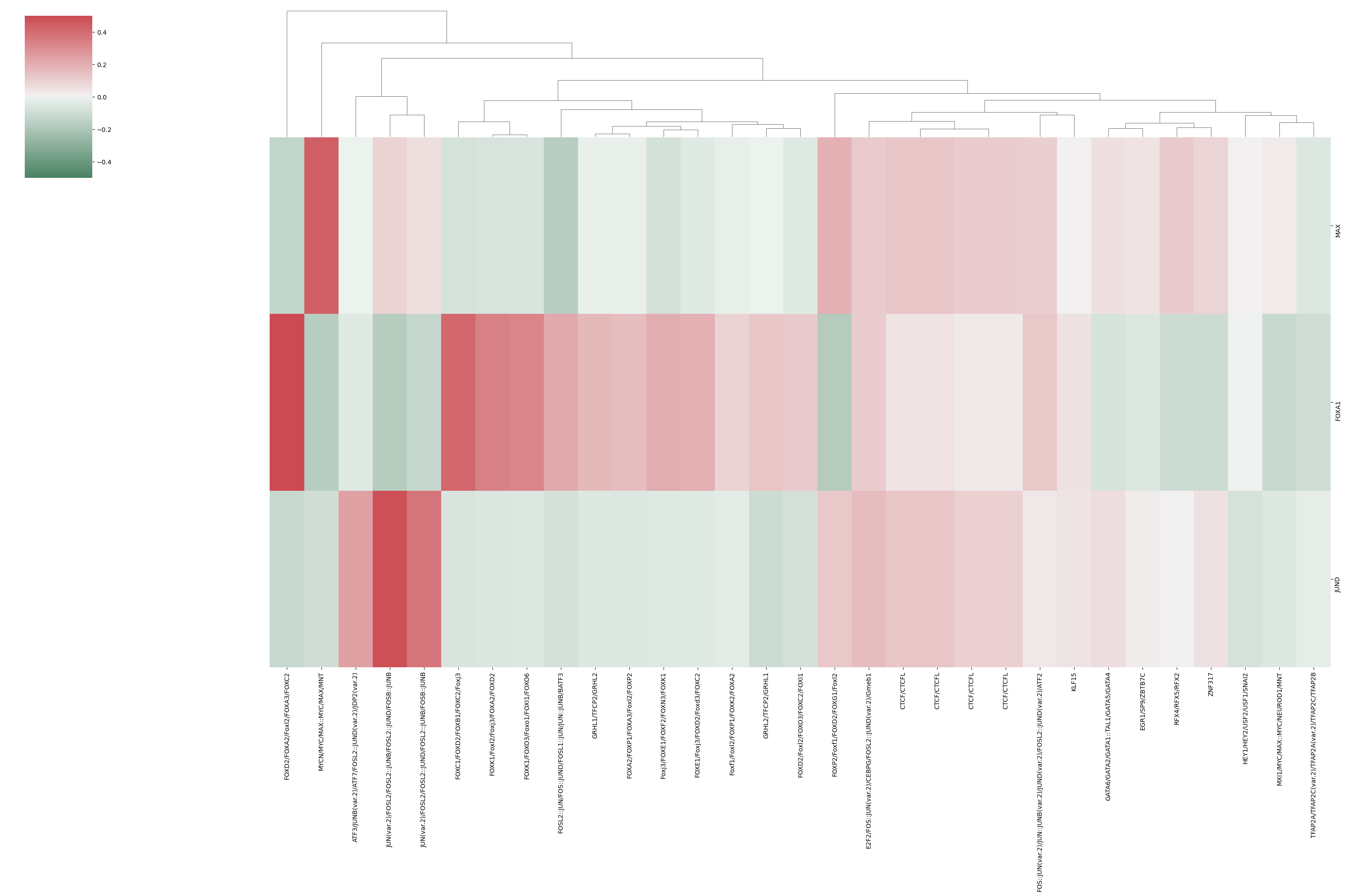
Retrieving the weights:
weights = model.final.weight.detach().cpu().numpy()

filters = ["filter"+str(i) for i in range(num_cnns)]
for i in annotation.keys():
    filters[int(i.split("filter")[-1])] = annotation[i]

weight_df = pd.DataFrame(weights, index=target_labels, columns=filters)
Visualizing the weights:
plt.figure(figsize=(15, 10))
# focus on annotated filters only
sns.clustermap(weight_df[[i for i in weight_df.columns if not i.startswith("filter")]],
               cmap=sns.diverging_palette(145, 10, s=60, as_cmap=True),
               row_cluster=False,
               figsize=(30, 20),
               vmax=0.5,
               vmin=-0.5)
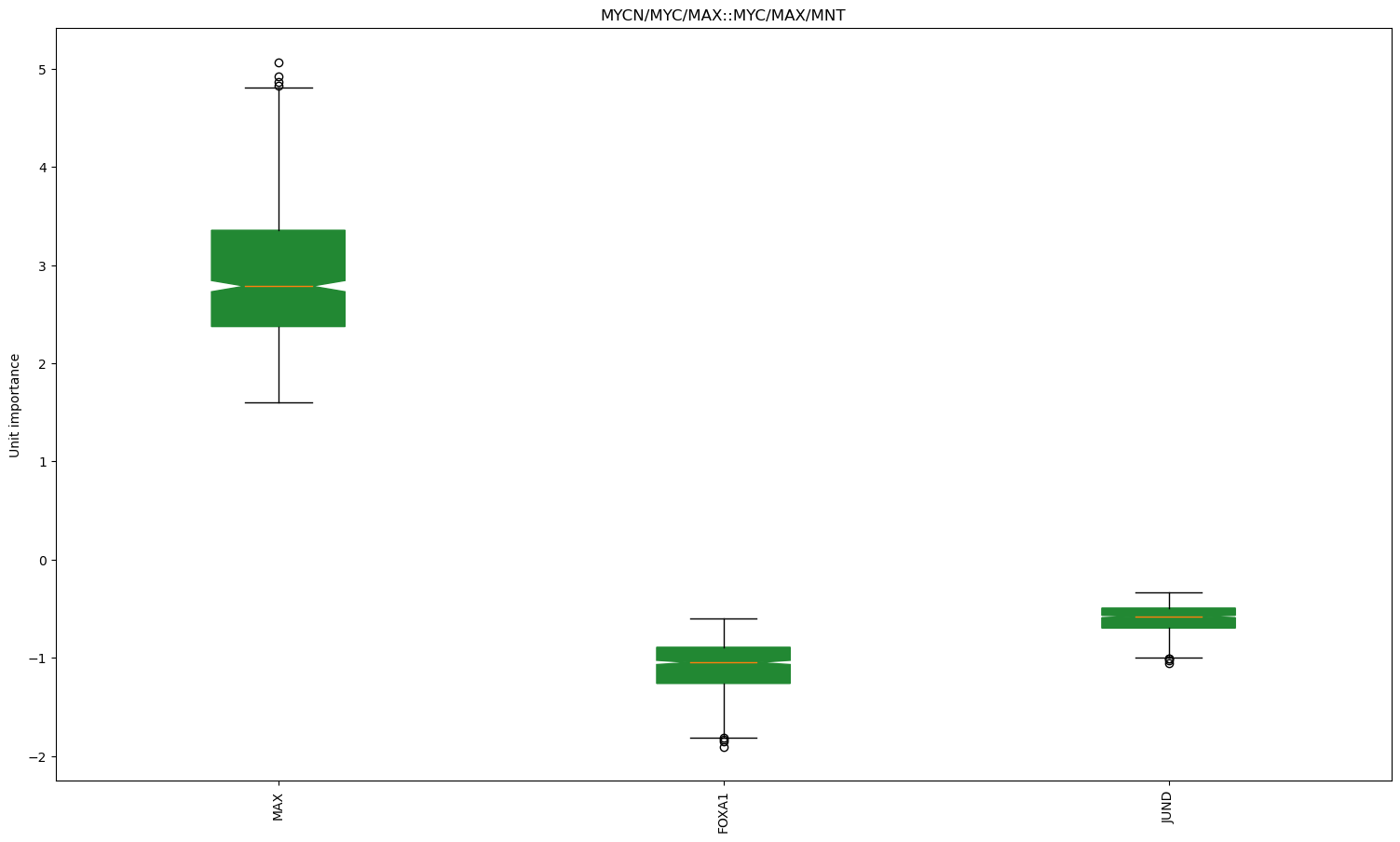
plt.show()Visualizing the MYC/MAX filter with the largest weight:
unit_outputs = interpretation.get_explainn_unit_outputs(data_loader, model, device)

best_filters = weight_df.idxmax(axis="columns")
best_myc_max_filter = weight_df.columns.get_loc(best_filters["MAX"])

unit_importance = interpretation.get_specific_unit_importance(activations,
                                                              model,
                                                              unit_outputs,
                                                              best_myc_max_filter,
                                                              target_labels)

filter_key = f"filter{best_myc_max_filter}"
title = annotation[filter_key] if filter_key in annotation.index else filter_key
fig, ax = plt.subplots()
datas = [filt_dat for filt_dat in unit_importance]
ax.boxplot(datas, notch=True, patch_artist=True, boxprops=dict(facecolor="#228833", color="#228833"))
fig.set_size_inches(18.5, 10.5)
plt.title(title)
plt.ylabel("Unit importance")
plt.xticks(range(1, len(target_labels)+1), target_labels)
plt.xticks(rotation=90)
plt.show()ExplaiNN's execution times are subject to 1) the size of the training dataset and 2) the number of units used. For an approximation to execution times for your dataset of interest please refer to Fig. 3D.
For a comprehensive guide on how to fully utilize ExplaiNN, including creating realistic backgrounds and analyzing the AI-TAC dataset, please refer to the tutorial provided here.
If you use ExplaiNN in your work, please cite:
ExplaiNN: interpretable and transparent neural networks for genomics
Gherman Novakovsky, Oriol Fornes, Manu Saraswat, Sara Mostafavi & Wyeth W. Wasserman
Genome Biololgy volume 24, Article number: 154 (2023). doi: 10.1186/s13059-023-02985-y.


