This package measures biological aging using data from the National Health and Nutrition Examination Survey (NHANES). The package uses published biomarker algorithms to calculate three biological aging measures: Klemera-Doubal Method (KDM) biological age, phenotypic age, and homeostatic dysregulation.
Citing the package
Kwon, D., Belsky, D.W. A toolkit for quantification of biological age from blood chemistry and organ function test data: BioAge. GeroScience 43, 2795–2808 (2021). https://doi.org/10.1007/s11357-021-00480-5
You can install the released version of BioAge from (https://github.com/dayoonkwon/BioAge) with:
install.packages("devtools")
devtools::install_github("dayoonkwon/BioAge")This serves as an example of training biologial aging measures using the
NHANES III (1988 - 1994) and projecting into NHANES IV (1999 - 2018)
dataset. It also provides documentation for fit parameters contained in
the BioAge package. The cleaned NHANES dataset is loaded as the
dataset NHANES3 and NHANES4. The original KDM bioage and phenoage
values are saved as kdm0 and phenoage0 as part of NHANES dataset.
library(BioAge) #topic of example
library(dplyr)I train in the NHANES III and project biological aging measures into the
NHANES IV by using the hd_nhanes, kdm_nhanes, and phenoage_nhanes
function of the BioAge package.
#HD using NHANES (separate training for men and women)
hd = hd_nhanes(biomarkers=c("albumin","alp","lncrp","totchol","lncreat","hba1c","sbp","bun","uap","lymph","mcv","wbc"))

#KDM bioage using NHANES (separate training for men and women)
kdm = kdm_nhanes(biomarkers=c("albumin","alp","lncrp","totchol","lncreat","hba1c","sbp","bun","uap","lymph","mcv","wbc"))

#phenoage uinsg NHANES
phenoage = phenoage_nhanes(biomarkers=c("albumin_gL","alp","lncrp","totchol","lncreat_umol","hba1c","sbp","bun","uap","lymph","mcv","wbc"))
Step 2: compare original KDM bioage and phenoage algorithms with algorithms composed with new biomarker set
The projected data and estimated models are saved as part of the list
structure. The dataset can be drawn by typing data. The model can be
drawn by typing fit.
#assemble NHANES IV dataset with projected biological aging measures for analysis
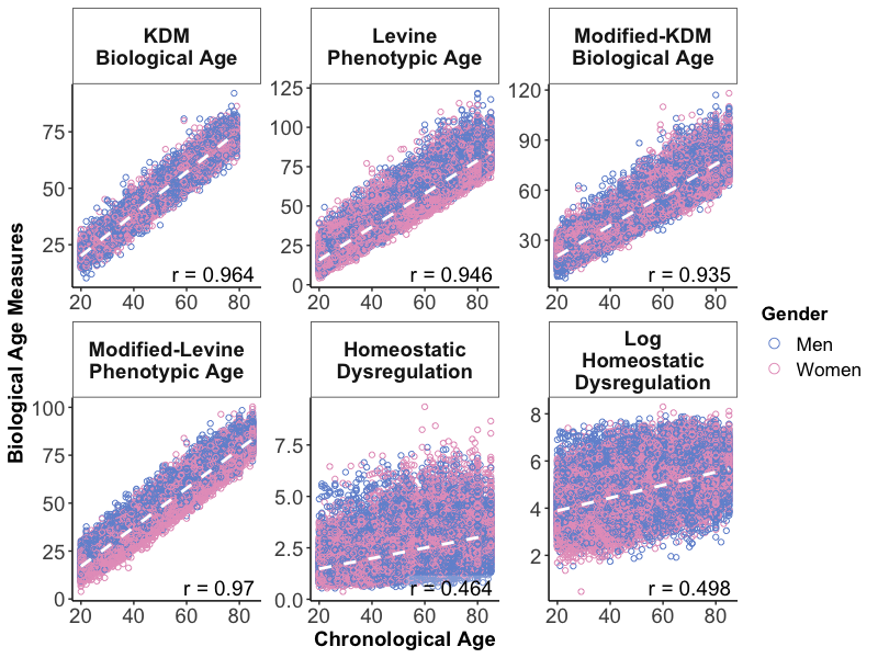
data = merge(hd$data, kdm$data) %>% merge(., phenoage$data)In the figure below, the graphs titled “KDM Biological Age” and “Levine Phenotypic Age” show measures based on the original biomarker sets published in Levine 2013 J Geron A and Levine et al. 2018 AGING. The remaining graphs shows the new measures computed with the biomarker set specified within this code.
#select biological age variables
agevar = c("kdm0","phenoage0","kdm","phenoage","hd","hd_log")

#prepare labels
label = c("KDM\nBiological Age",
          "Levine\nPhenotypic Age",
          "Modified-KDM\nBiological Age",
          "Modified-Levine\nPhenotypic Age",
          "Homeostatic\nDysregulation",
          "Log\nHomeostatic\nDysregulation")

#plot age vs bioage
plot_ba(data, agevar, label)The figure plots associations among the different biological aging measures. Cells below the diagonal show scatter plots of the measures listed above the cell (x-axis) and to the right (y-axis). Cells above the diagonal show the Pearson correlations for the measures listed below the cell and to the left. For this analysis, KDM Biological Age and Levine Phenotypic Age measures are differenced from chronological age (i.e. plotted values = BA-CA).
#select biological age variables
agevar = c("kdm_advance0","phenoage_advance0","kdm_advance","phenoage_advance","hd","hd_log")

#prepare lables
#values should be formatted for displaying along diagonal of the plot
#names should be used to match variables and order is preserved
label = c(
  "kdm_advance0"="KDM\nBiological Age\nAdvancement",
  "phenoage_advance0"="Levine\nPhenotypic Age\nAdvancement",
  "kdm_advance"="Modified-KDM\nBiological Age\nAdvancement",
  "phenoage_advance"="Modified-Levine\nPhenotypic Age\nAdvancement",
  "hd" = "Homeostatic\nDysregulation",
  "hd_log" = "Log\nHomeostatic\nDysregulation")

#use variable name to define the axis type ("int" or "float")
axis_type = c(
  "kdm_advance0"="float",
  "phenoage_advance0"="float",
  "kdm_advance"="float",
  "phenoage_advance"="flot",
  "hd"="flot",
  "hd_log"="float")

#plot BAA corplot
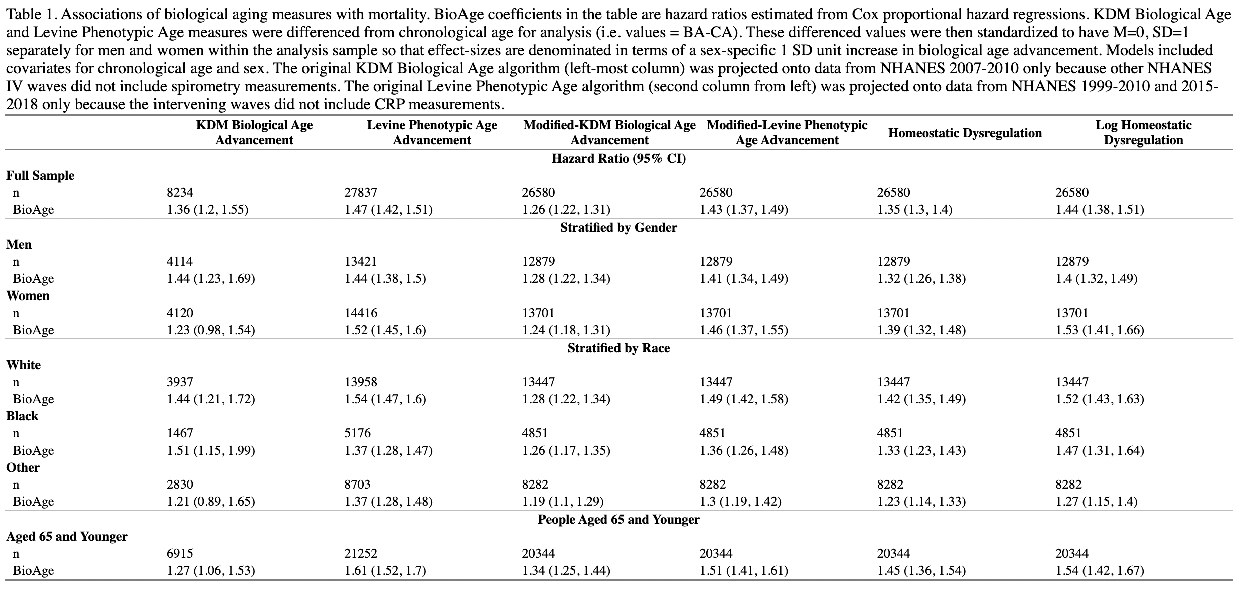
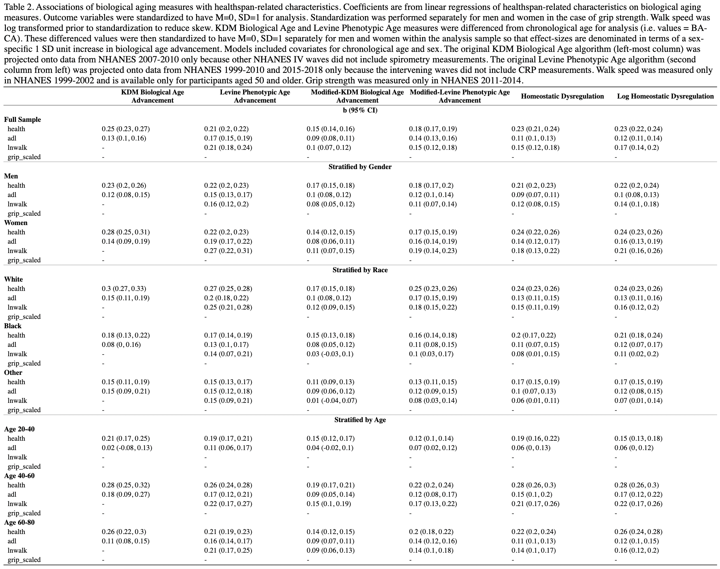
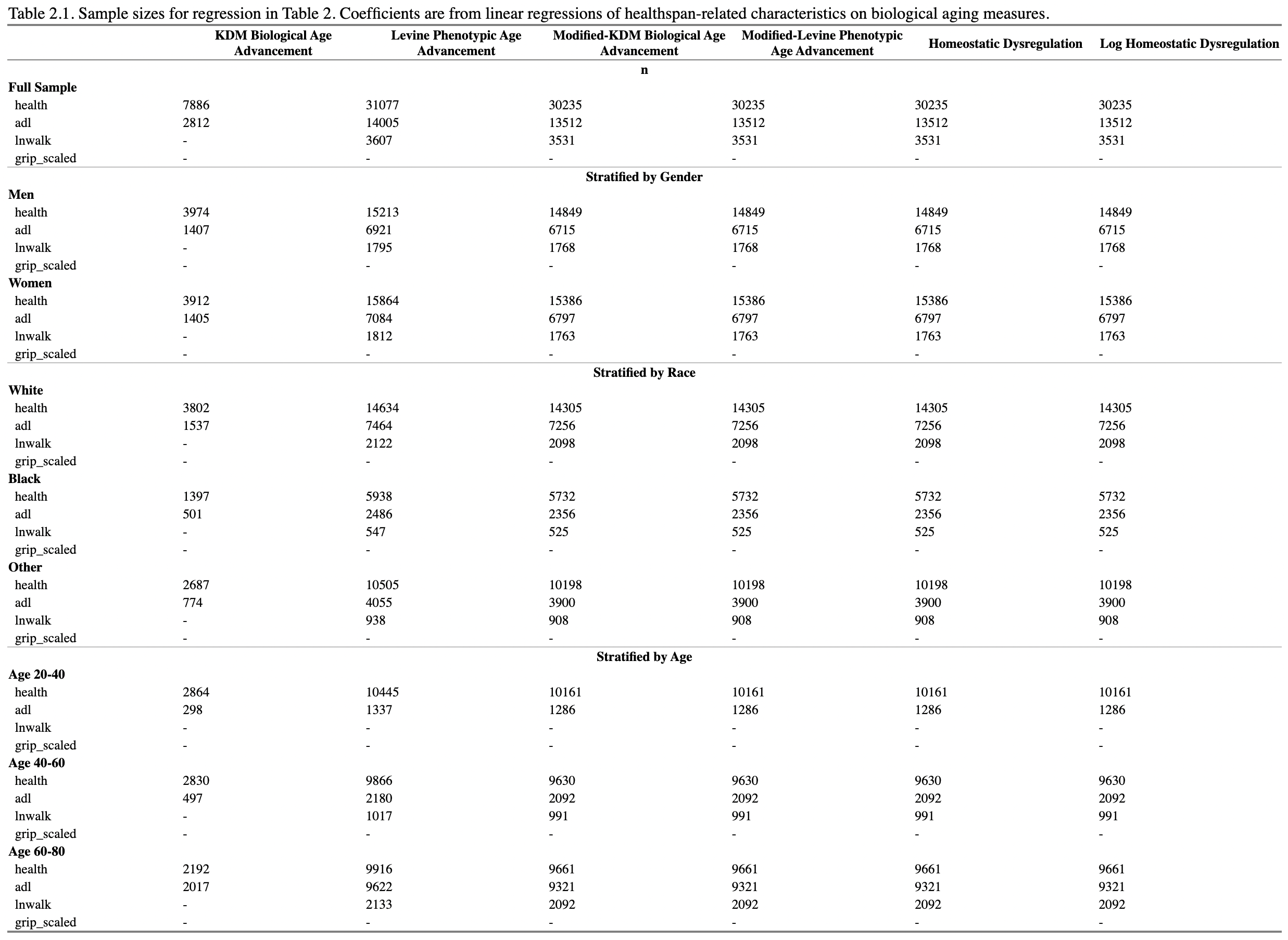
plot_baa(data,agevar,label,axis_type)table_surv(data, agevar, label)The linear regression models and sample sizes in “Table 2” and “Table 3”
below are saved as part of the list structure. Regression model can be
drawn by typing table. Sample size can be drawn by typing n.
table2 = table_health(data,agevar,outcome = c("health","adl","lnwalk","grip_scaled"), label)

#pull table
table2$table#pull sample sizes
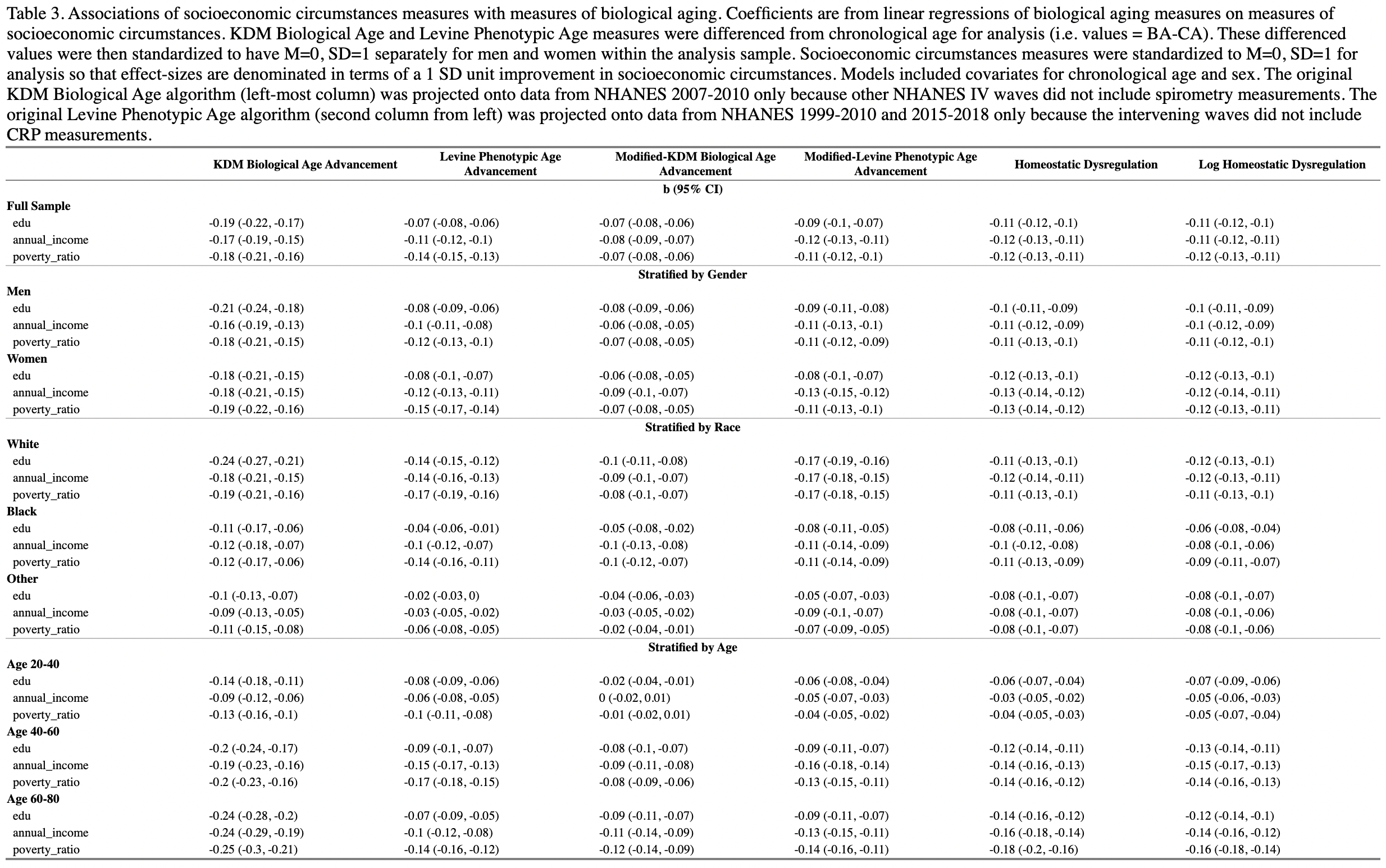
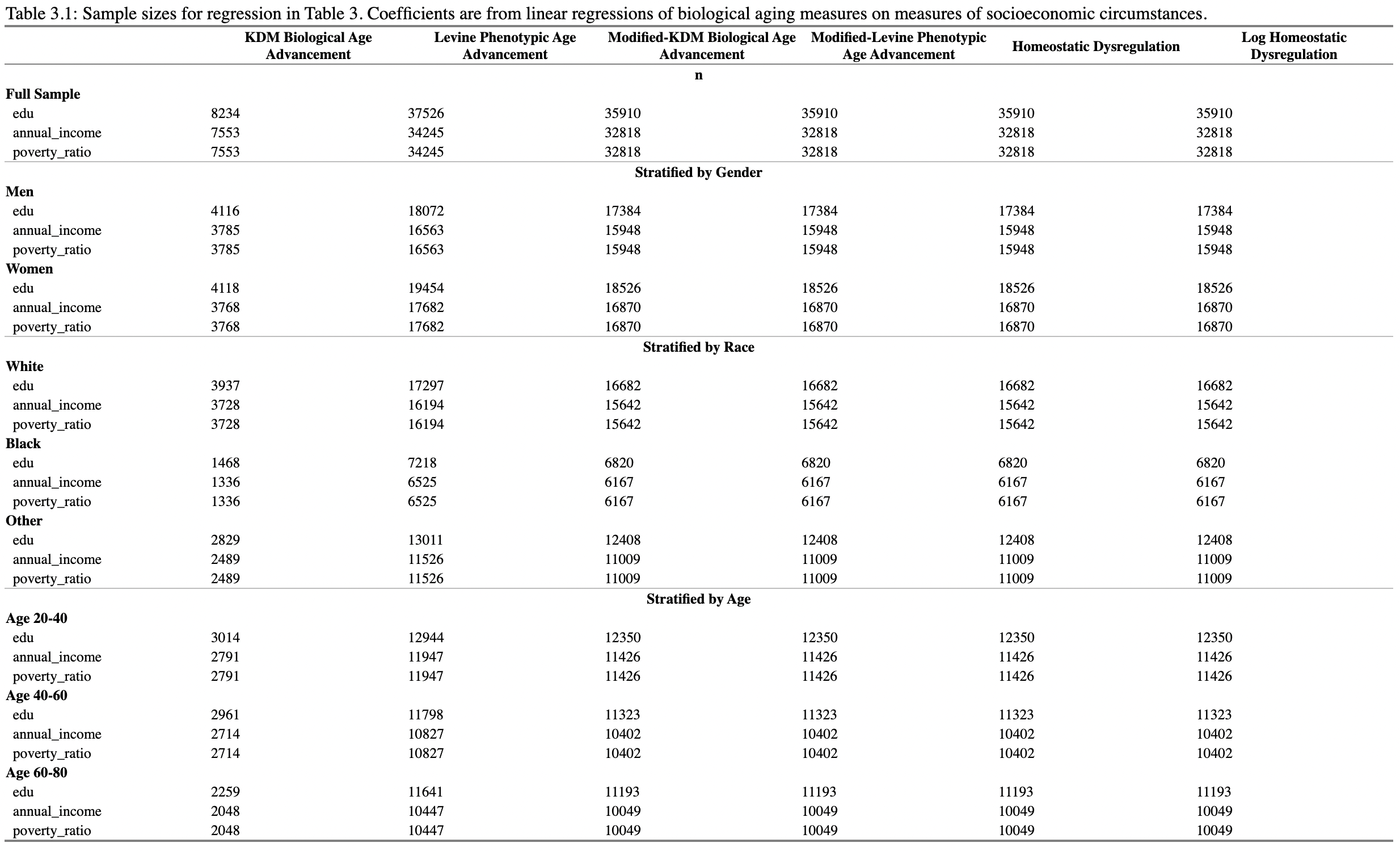
table2$ntable3 = table_ses(data,agevar,exposure = c("edu","annual_income","poverty_ratio"), label)
#pull table
table3$table#pull sample sizes
table3$nIn this example, the projection dataset is from the CALERIE randomized
controlled trial (data are not included in the package). For this
analysis, CALERIE data were previously cleaned and units of measure and
variable names were harmonized to match the NHANES data included with
the package. All algorithms were trained using the NHANES III data and
projected into the CALERIE using the hd_calc, kdm_calc, and
phenoage_calc functions of the BioAge package.
For HD, the constructed variable is based on a malhanobis distance statistic, which is theoretically the distance between observations and a hypothetically healthy, young cohort. In this example, I train separately for men and women who are between the ages of 20 and 30 and not pregnant, and have observe biomarker data within clinically acceptable distributions. For clinical guidelines, I relied upon the ranges reported by the Mayo Clinic website.
#The CALERIE dataset is loaded from my local drive that has previously been downloaded and cleaned
#projecting HD into the CALERIE using NHANES III (seperate training for gender)
hd_fem = hd_calc(data = CALERIE %>%
                      filter(gender == 2)%>%
                      mutate(lncrp = log(crp)),
                    reference = NHANES3_CLEAN %>%
                      filter(gender == 2)%>%
                      mutate(lncrp = log(crp)),
                    biomarkers=c("albumin","alp","lncrp","totchol","lncreat","hba1c","sbp","bun","uap","lymph","mcv","wbc"))

hd_male = hd_calc(data = CALERIE %>%
                       filter(gender == 1)%>%
                       mutate(lncrp = log(crp)),
                     reference = NHANES3_CLEAN %>%
                       filter(gender == 1)%>%
                       mutate(lncrp = log(crp)),
                     biomarkers=c("albumin","alp","lncrp","totchol","lncreat","hba1c","sbp","bun","uap","lymph","mcv","wbc"))

#pull the HD dataset
hd_data = rbind(hd_fem$data, hd_male$data)Having estimated biological aging models using NHANES III in “Step 1”, I
can project KDM bioage and phenoage into the CALERIE data by running
kdm_calc and phenoage_calc and supplying a fit argument.
#projecting KDM bioage into the CALERIE using NHANES III (seperate training for gender)
kdm_fem = kdm_calc(data = CALERIE %>%
                        filter (gender ==2),
                      biomarkers=c("albumin","alp","lncrp","totchol","lncreat","hba1c","sbp","bun","uap","lymph","mcv","wbc"),
                   fit = kdm$fit$female,
                   s_ba2 = kdm$fit$female$s_b2)

kdm_male = kdm_calc(data = CALERIE %>%
                         filter (gender ==1),
                       biomarkers=c("albumin","alp","lncrp","totchol","lncreat","hba1c","sbp","bun","uap","lymph","mcv","wbc"),
                   fit = kdm$fit$male,
                   s_ba2 = kdm$fit$male$s_b2)

#pull the KDM dataset
kdm_data = rbind(kdm_fem$data, kdm_male$data)phenoage_CALERIE = phenoage_calc(data = CALERIE,
biomarkers = c("albumin_gL","alp","lncrp","totchol","lncreat_umol","hba1c","sbp","bun","uap","lymph","mcv","wbc"),
fit = phenoage$fit)
phenoage_data = phenoage_CALERIE$data
#pull the full dataset
newdata = left_join(CALERIE, hd_data[, c("sampleID", "hd", "hd_log")], by = "sampleID") %>%
left_join(., kdm_data[, c("sampleID", "kdm", "kdm_advance")], by = "sampleID") %>%
left_join(., phenoage_data[, c("sampleID","phenoage","phenoage_advance")], by = "sampleID") Summary statistics of calculated biological aging measures for the CALERIE at pre-intervention baseline
summary(newdata %>% filter(fu==0) %>% select(kdm, phenoage, hd, hd_log))
#>       kdm           phenoage           hd             hd_log
#>  Min.   :22.37   Min.   :11.97   Min.   :0.8641   Min.   :2.097
#>  1st Qu.:31.79   1st Qu.:27.41   1st Qu.:2.2555   1st Qu.:4.695
#>  Median :38.70   Median :32.99   Median :2.7147   Median :5.229
#>  Mean   :37.43   Mean   :32.64   Mean   :2.9256   Mean   :5.324
#>  3rd Qu.:42.84   3rd Qu.:38.14   3rd Qu.:3.4509   3rd Qu.:6.023
#>  Max.   :50.60   Max.   :50.58   Max.   :7.9852   Max.   :8.797
#>  NA's   :13      NA's   :13      NA's   :13       NA's   :13