GeoGaussian: Geometry-aware Gaussian Splatting for Scene Rendering (ECCV 2024)

📖 Abstract

During the Gaussian Splatting optimization process, the scene geometry can gradually deteriorate if its structure is not deliberately preserved, especially in non-textured regions such as walls, ceilings, and furniture surfaces. This degradation significantly affects the rendering quality of novel views that deviate significantly from the viewpoints in the training data. To mitigate this issue, we propose a novel approach called GeoGaussian. Based on the smoothly connected areas observed from point clouds, this method introduces a novel pipeline to initialize thin Gaussians aligned with the surfaces, where the characteristic can be transferred to new generations through a carefully designed densification strategy. Finally, the pipeline ensures that the scene geometry and texture are maintained through constrained optimization processes with explicit geometry constraints. Benefiting from the proposed architecture, the generative ability of 3D Gaussians is enhanced, especially in structured regions. Our proposed pipeline achieves state-of-the-art performance in novel view synthesis and geometric reconstruction, as evaluated qualitatively and quantitatively on public datasets.

3DGS | LightGS | GeoGaussian(Ours)

Comparisons of novel view rendering on public datasets. At some challenging viewpoints having bigger differences in translation and orientation motions compared with training views, 3DGS and LightGS have issues with photorealistic rendering.

📋 TODO Lists

🚀 Geometry-aware Strategies

A parameterization with explicit geometry meaning for thin 3D Gaussians is employed in our carefully designed initialization and densification strategies} to establish reasonable 3D Gaussian models.
A geometrically consistent constraint is proposed to encourage thin Gaussians to align with the smooth surfaces.

💾 Dataset

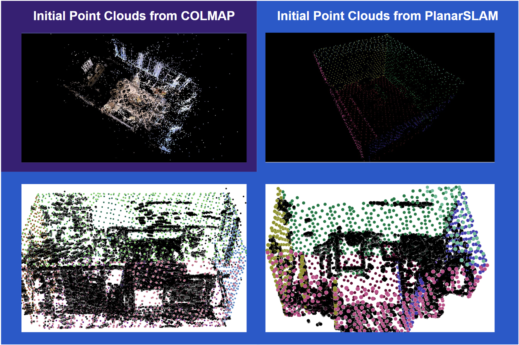
Based on the SLAM method, PlanarSLAM, we create new point clouds rather then using results of COLMAP for experiments.

New Features of this type of input:

Points lying on the non-textured regions
Global plane instances that are represented in different colors
Surface normal vector of each planar point

The subdataset can be obtained via Replica (PlanarSLAM), TUM RGB-D (PlanarSLAM), ICL NUIM (PlanarSLAM). Then you need to place the raw dataset images in the results folder. The raw images can be obtained via Replica, TUM RGB-D, ICL NUIM.

For each sequence, the structure is organized as follows

Replica_r2
	|______PointClouds.ply          # sparse point clouds from the SLAM system
 	|______KeyFrameTrajectory2.txt  # camera poses from the SLAM system
  	|______results                  # folder for all raw images

our code provides the interface to deal with the type of data format.

🎓 Baseline

1. Gaussian-Splatting with Planar Point Clouds Repo

🔧 Setup of GeoGaussian

1. Clone the repo.

# https
git clone https://github.com/yanyan-li/GeoGaussian
# or ssh
git clone git@github.com:yanyan-li/GeoGaussian.git

2. Environment setup.

If you have an environment used for 3dgs, use it. If not, please refer to the environment configuration of 3DGS environment The environment.yml file for 3DGS has been provided in our repo.

Additionally, you also need to install the open3d scipy matplotlib pillow libraries.

# If you have already installed the 3dgs environment,
# please activate the environment and execute the following command :
conda activate gaussian_splatting
pip install open3d scipy matplotlib pillow

3. Download the demo dataset

Create a new data folder
Download the file (Replica OFF2).
Unzip it to data folder.

4. Run the codes

In order to run our code, you should specify the path of the dataset which should include the KeyFrameTrajectory.txt file or sparse folder and specify the sparsity of the images that is the interval between the input images.

# python train.py -s [path_to_dataset] --sparse_num [N]( 1 ==> 100% images, 5 ==> 20% images)

Run demo:

python train.py -s data/Replica-OFF2 --sparse_num 1

Then you will find that the output folder has a specific xxxxxxxx-x directory, as well as depth and rgb directories, which respectively store the RGB and depth images rendered during the training process.

📊 Results

Methods
Data

3DGS

LightGS

GeoGaussian(Ours)

PSNR↑
SSIM↑
LPIPS↓

30.49

33.98

37.45

37.60

30.54

34.06

37.72

38.44

31.65

35.17

38.00

38.24

0.932

0.951

0.964

0.965

0.932

0.951

0.965

0.967

0.937

0.957

0.968

0.979

0.051

0.036

0.029

0.028

0.051

0.035

0.028

0.025

0.041

0.027

0.022

0.021

PSNR↑
SSIM↑
LPIPS↓

31.53

35.82

38.53

38.70

31.54

35.93

38.78

39.07

32.13

36.81

38.84

39.14

0.935

0.959

0.968

0.935

0.959

0.968

0.943

0.963

0.969

0.970

0.050

0.031

0.028

0.029

0.049

0.031

0.027

0.028

0.041

0.025

0.024

OFF3

PSNR↑
SSIM↑
LPIPS↓

30.90

33.86

36.26

36.56

30.93

33.90

36.38

36.63

31.62

33.91

36.42

36.66

0.928

0.946

0.958

0.959

0.928

0.947

0.958

0.958

0.938

0.953

0.963

0.964

0.052

0.040

0.037

0.036

0.052

0.040

0.036

0.037

0.040

0.032

0.029

OFF4

PSNR↑
SSIM↑
LPIPS↓

29.5

32.98

37.70

38.48

29.51

32.97

37.95

38.59

31.90

34.61

38.30

38.74

0.920

0.941

0.962

0.964

0.920

0.941

0.962

0.964

0.936

0.953

0.966

0.967

0.070

0.049

0.037

0.035

0.070

0.049

0.036

0.036

0.050

0.036

0.030

0.031

Avg.

PSNR↑
SSIM↑
LPIPS↓

30.62

34.16

37.49

37.84

30.63

34.22

37.71

38.18

31.83

35.13

38.18

38.20

0.929

0.949

0.964

0.929

0.950

0.964

0.939

0.957

0.967

0.970

0.056

0.039

0.032

0.056

0.039

0.032

0.043

0.030

0.026

Table I. Comparison of rendering on the Replica dataset. ↓ indicates the lower the better, ↑ indicates the higher the better. The best score is in bold and italic. The second best score is in italic.

methods		R0	R1	R2	OFF0	OFF1	OFF2	OFF3	OFF4	Avg.
3DGS GeoGaussian (Ours)	mean (m) std (m)	0.026	0.025	0.042	0.017	0.019	0.039	0.032	0.032	0.029
	mean (m) std (m)	0.066	0.081	0.146	0.050	0.055	0.201	0.066	0.112	0.097
	mean (m) std (m)	0.018	0.014	0.015	0.020	0.029	0.013	0.018	0.014	0.018
	mean (m) std (m)	0.032	0.016	0.028	0.042	0.067	0.024	0.020	0.023	0.031

Table II. Comparison of reconstruction performance on the Replica dataset. Based on the ground truth mesh models provided by the Replica dataset, we align these mesh models with point clouds from Gaussian models, where we randomly sample three points in each Gaussian ellipsoid.

⭕️ Acknowledgment

This project is based on 3DGS and relies on data provided by PlanarSLAM work. Thanks for the contribution of the open source community.

📋 License

This project is released under the Gaussian-Splatting License.

✉️ Citation

If you find this project useful in your research, please consider cite:

BibTex

@article{li2024geogaussian,
  title={GeoGaussian: Geometry-aware Gaussian Splatting for Scene Rendering},
  author={Li, Yanyan and Lyu, Chenyu and Di, Yan and Zhai, Guangyao and Lee, Gim Hee and Tombari, Federico},
  journal={arXiv preprint arXiv:2403.11324},
  year={2024}
}

wlt027/GeoGaussian

GeoGaussian: Geometry-aware Gaussian Splatting for Scene Rendering (ECCV 2024)

📖 Abstract

📋 TODO Lists

🚀 Geometry-aware Strategies

💾 Dataset

🎓 Baseline

🔧 Setup of GeoGaussian

1. Clone the repo.

2. Environment setup.

3. Download the demo dataset

4. Run the codes

📊 Results

⭕️ Acknowledgment

📋 License

✉️ Citation