BinghamNLL

Overview

The repository contains the implementation of Bingham distribution's Negative Log-Likelihood(NLL) loss function.

Our paper is accepted by 2023 IEEE International Conference on Robotics and Automation (ICRA) under the title "A Probabilistic Rotation Representation for Symmetric Shapes With an Efficiently Computable Bingham Loss Function", by Hiroya Sato, Takuya Ikeda, and Koichi Nishiwaki.

The paper and video are available:

arXiv: http://arxiv.org/abs/2305.18947
YouTube: https://www.youtube.com/watch?v=UQEEdeevpDo

If you use our BinghamNLL in your work, please cite as follows:

@inproceedings{hiroya_binghamnll_2023,
   author={Hiroya Sato and Takuya Ikeda and Koichi Nishiwaki},
   title={{A Probabilistic Rotation Representation for Symmetric Shapes With an Efficiently Computable Bingham Loss Function}},
   booktitle={{2023 International Conference on Robotics and Automation (ICRA)}},
   year={2023},
   month={May},
   pages={6923-6929},
}

How to install

git clone https://github.com/woven-planet/BinghamNLL.git
cd BinghamNLL
git submodule update --init --recursive
python3 -m venv venv
source venv/bin/activate
pip install --upgrade pip
pip install -r requirements.txt
pip install -r requirements.cpu.txt
pip install -r requirements.submodule.txt

If you'd like to use GPU, please modify requirements.gpu.txt based on your environment. Then, please use it instead of the above requirements.cpu.txt.

To check successful installation,

python3 -m unittest test/test_bingham_loss.py

Try example codes

Run the following code:

python3 optim_params.py -N 20 --seed 593

without --dryrun option,
- After running it, you will get outputs/mats/hhmmss_yyyyMMdd.mat.
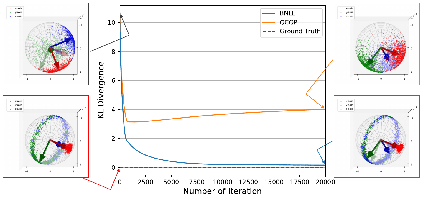
- The visualization of optimized distribution can be found in outputs/pngs/*.png
  - init.png: the initial distribution of optimization.
  - truth.png: the distribution that sampled points are from.
    - init.png and truth.png are generated as soon as optim_params.py is called.
  - bnll.png: the resulting distribution optimized using Bingham NLL loss.
  - qcqp.png: the resulting distribution optimized using QCQP Loss (Peretroukhin et al., 2020)
- The optimization result will be saved even if you send Ctrl-C during the optimization.
- The visualized results are saved in outputs/pdfs/*.pdf
with --show option the visualized results are shown after optimization.
You can change the number of sample points by specifying N (default = 20).
You can change the truth distribution by specifying seed (default = None).
- Here we set seed = 593 for example. This produces the axis symmetric distribution.
- We found seed = 593, 784, 847, 914, 949 generates the symmetric distribution.

(Optional)

Visualized results can be created from outputs/mats/*.mat after running optim_params.py.

Run the following code:

python3 visualize_mats.py

then they are saved in outputs/pdfs/*.pdf

You can find the result pdf that looks like the following:

Unittest

python3 -m unittest

API Documentation

To get api documenataion, please install sphinx and build it based on the below.

pip install -r requirements.docs.txt
cd docs
make html

Then, index.html should be generated in docs/_build/html directory.

About This Project and Us

This work has been done at Woven by Toyota, Inc. A part of the work is the result of Summer Internship Program.

Hiroya Sato is with Department of Mechano-Informatics, Graduate School of Information Science and Technology, The University of Tokyo.

Takuya Ikeda and Koichi Nishiwaki are with the Woven by Toyota, Inc.

Acknowledgement

The visualization of Bingham distribution was supported by Ching-Hsin Fang and Duy-Nguyen Ta in Toyota Research Institute. We'd like to express our deep gratitude to them.

License

Apache License 2.0