microbiomer

The goal of microbiomer is to provide a small set of tools to more seamlessly integrate tools/functions from both the phyloseq and tidyverse-packages.

Note this is a package in development; although the functions were not yet tested extensively within the context of this package, they were tested across several projects as source code. Nevertheless, use these functions at your own risk and please file a report if you come across issues.

Installation

You can install the development version from GitHub with:

# install.packages("devtools")
devtools::install_github("wsteenhu/microbiomer")

The package has not been submitted to CRAN.

Example

Load packages

library(microbiomer); library(phyloseq)
library(tidyverse)
#> ── Attaching packages ─────────────────────────────────────── tidyverse 1.3.0 ──
#> ✓ ggplot2 3.3.3     ✓ purrr   0.3.4
#> ✓ tibble  3.0.6     ✓ dplyr   1.0.4
#> ✓ tidyr   1.1.2     ✓ stringr 1.4.0
#> ✓ readr   1.3.1     ✓ forcats 0.5.1
#> ── Conflicts ────────────────────────────────────────── tidyverse_conflicts() ──
#> x dplyr::filter() masks stats::filter()
#> x dplyr::lag()    masks stats::lag()

Load data

data(ps_NP)
ps_NP
#> phyloseq-class experiment-level object
#> otu_table()   OTU Table:         [ 1793 taxa and 287 samples ]
#> sample_data() Sample Data:       [ 287 samples by 5 sample variables ]
#> tax_table()   Taxonomy Table:    [ 1793 taxa by 8 taxonomic ranks ]

The package includes nasopharyngeal microbiota data collected at 1 week, 1 month and 1 year of life. For more information, see ?ps_NP.

Convert

ps_NP_RA <- otu_table(ps_NP) %>%
  to_RA() 

ps_NP_RA[1:5,1:3] # depict example
#> OTU Table:          [5 taxa and 3 samples]
#>                      taxa are rows
#>                         121142010012 121144010012 121150010012
#> Moraxella_2             0.0002340276 0.0002837819 0.6826699800
#> Corynebacterium_5       0.0000000000 0.1827082249 0.0743064326
#> Dolosigranulum_pigrum_7 0.3214870783 0.2691671002 0.2292948222
#> Staphylococcus_3        0.0322958109 0.0283308897 0.0001018454
#> Haemophilus_9           0.0000000000 0.0004256728 0.0000000000

to_RA converts the otu_table-object nested within a phyloseq-object into a total-sum-scaled table (relative abundances instead of raw reads).

Filter

ps_NP %>% ntaxa()
#> [1] 1793

ps_NP %>%
  pres_abund_filter()
#> A total of 224 ASVs were found to be present at or above a level of confident detection (0.1% relative abundance) in at least 2 samples (n = 1569 ASVs excluded).
#> phyloseq-class experiment-level object
#> otu_table()   OTU Table:         [ 224 taxa and 287 samples ]
#> sample_data() Sample Data:       [ 287 samples by 5 sample variables ]
#> tax_table()   Taxonomy Table:    [ 224 taxa by 8 taxonomic ranks ]

Use a filter described by Subramanian et al. (Nature, 2014) to filter phyloseq-objects.

Extract metadata

ps_NP %>%
  meta_to_df() %>%
  head()
#>      sample_id seq_id visit_name age birth_mode bf_group_3m_yn
#> 1 121142010012   M001         w1   8        vag              1
#> 2 121144010012   M001         m1  30        vag              1
#> 3 121150010012   M001         y1 364        vag              1
#> 4 121142010032   M003         w1   7        vag              1
#> 5 121144010032   M003         m1  32        vag              1
#> 6 121150010032   M003         y1 361        vag              1

meta_to_df() convers the sample_data()-objects within a phyloseq-object into a tidyverse-formatted data table. Also try otu_tab_to_df() and ps_to_df()

Prepare for plotting

ps_NP %>%
  prep_bar(n = 5) %>%
  head()
#> # A tibble: 6 x 8
#>   sample_id  seq_id visit_name   age birth_mode bf_group_3m_yn OTU         value
#>   <fct>      <chr>  <ord>      <dbl> <chr>      <fct>          <fct>       <dbl>
#> 1 121142010… M001   w1             8 vag        1              *Moraxella…     7
#> 2 121142010… M001   w1             8 vag        1              *Staphyloc…   966
#> 3 121142010… M001   w1             8 vag        1              *Corynebac…     0
#> 4 121142010… M001   w1             8 vag        1              *Dolosigra…  9616
#> 5 121142010… M001   w1             8 vag        1              *Haemophil…     0
#> 6 121142010… M001   w1             8 vag        1              Residuals   19322

The function prep_bar() converts your phyloseq-object into an object that can be readily used for plotting. It includes all metadata-columns, a column ‘OTU’ (with formatted OTU-names) and a column ‘value’ with read counts/relative abundances (depending on the format of the otu_table).

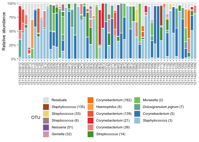
Barplot

ps_NP %>% 
  subset_samples(., birth_mode == "vag" & visit_name == "w1") %>% # select samples
  to_RA %>%
  create_bar()

Note this plotting function can be used in conjunction with other ggplot2-functions/extensions, such as coord_flip()/ggforce::facet_col() and facet_wrap().