Spatial-CITE-seq

This repository aims to share the raw data processing and visualization codes used in Hiplex_proteome sequencing project.

This repository includes the main R scripts used for the visualization of the sequencing data of RNA and protein, including clustering, Differential expression gene/protein analysis, integrated analysis, etc.

Abstract

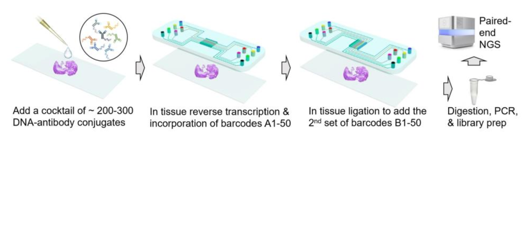
Spatial-CITE-seq is a spatial multiomic sequencing technique that can also be directly applied for transcriptome and hiplex protein sequencing. We have successfully demonstrated spatial omics sequencing of mouse and human sections at cellular level (25μm pixel size) with high coverage of genes (>1,000 genes per pixel) and proteins (200-300 proteins per pixel).

Data processing

1. Raw Fastq data processing using ST pipeline and generate expression matrix

We did the illumina pair-end 100 sequencing using Novaseq 6000 and pool two samples (tissue sections) for each sequencing lane.

The Spatial-CITE-seq Raw fastq file

Read 1: Contains the cDNA sequence or protein barcode

Read 2: Contains the spatial Barcode A, Barcode B and UMIs

Reformat Fastq Read 2 file

To run ST pipeline, the Read 2 sequence needs to be reformated, see following figure. Due to different experimental design, the Read 2 of DBiT-seq is equal to the "Read 1" in ST pipeline, while Read 1 will be the "Read 2".

To reformat the Raw data, run the fastq_process.py in Rawdata_processing folder and gzip the resulted fastq file to save space:

python fastq_process.py
gzip sample_R2_processed.fastq

The reformated data was processed following ST pipeline.

Run ST pipeline

Run st_pipeline.sh to start the ST pipeline: The input is processed_R2.fastq.gz and Raw R1.fastq.gz. It also requires a "spatial_barcodes_index.txt" to decode the spatial location information. Genome references and annotatation files were aslo needed.

#!/bin/bash

# FASTQ reads
FW=PATH_TO_PROCESSED_R2/sample_R2_processed.fastq.gz
RV=PATH_TO_R1/R1.fastq.gz

# References for mapping and annotation 
MAP=PATH_TO_ALIGNMENT_REF/Dropseq_Alignment_References/mm10/
ANN=PATH_TO_ALIGNMENT_REF_GTF/Dropseq_Alignment_References/mm10/mm10.gtf

# Barcodes settings
ID=PATH_TO_BARCODE_INDEX/spatial_barcodes_index.txt 

# Output folder and experiment name
OUTPUT=PATH_TO_OUTPUT/st_pipeline_new/
mkdir -p PATH_TO_OUTPUT/st_pipeline_new/

TMP=PATH_TO_TEMP/st_pipeline_new/tmp
mkdir -p PATH_TO_TEMP/st_pipeline_new/tmp

# Do not add / or \ to the experiment name
EXP=FFPE-2

# Running the pipeline
st_pipeline_run.py \
  --output-folder $OUTPUT \
  --ids $ID \
  --ref-map $MAP \
  --ref-annotation $ANN \
  --expName $EXP \
  --htseq-no-ambiguous \
  --verbose \
  --log-file $OUTPUT/${EXP}_log.txt \
  --allowed-kmer 5 \
  --mapping-threads 20 \
  --temp-folder $TMP \
  --no-clean-up \
  --umi-start-position 16 \
  --umi-end-position 26 \
  --overhang 0 \
  --min-length-qual-trimming 10 \
  $FW $RV

Convert Ensemble to Gene Names

Then, Run converttoname.sh to annotate the resulting FFPE2_stdata.tsv.

#!/bin/bash

tsv_E=FFPE-2_stdata.tsv
path_to_annotation_file=PATH_TO_ALIGNEMNT/Dropseq_Alignment_References/mm10/mm10.gtf
convertEnsemblToNames.py $tsv_E --annotation $path_to_annotation_file --output FFPE-2_exp_matrix.tsv

Now, the expression matrix is successfully generated. The row names are "XxY" location for each pixel, and columne names are Genes.

2. Identify useful pixels (pixel on tissue) from microscope image using Matlab

Useful pixels were generated from the Matlab script. Basically, it divide the real tissue microscope image into 50x50 small sqaures which match with DBiT-seq pixels. Then, the intensity inside each pixel was calculated and only pixels have signals above a threashold will be selected.

There two steps: To run the Matlab script "Pixel_identification.m"

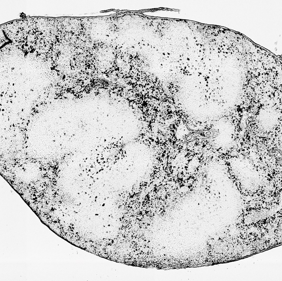
Use Photoshop or other photo editing software to crop the microscope image into exactly the size of the DBiT-seq covering area. For example, the upperleft of the image should be the 1x1 pixel of DBiT-seq, and the lowerright is the 50x50. No space is allowed. See "FFPE-2.jpg" for example.

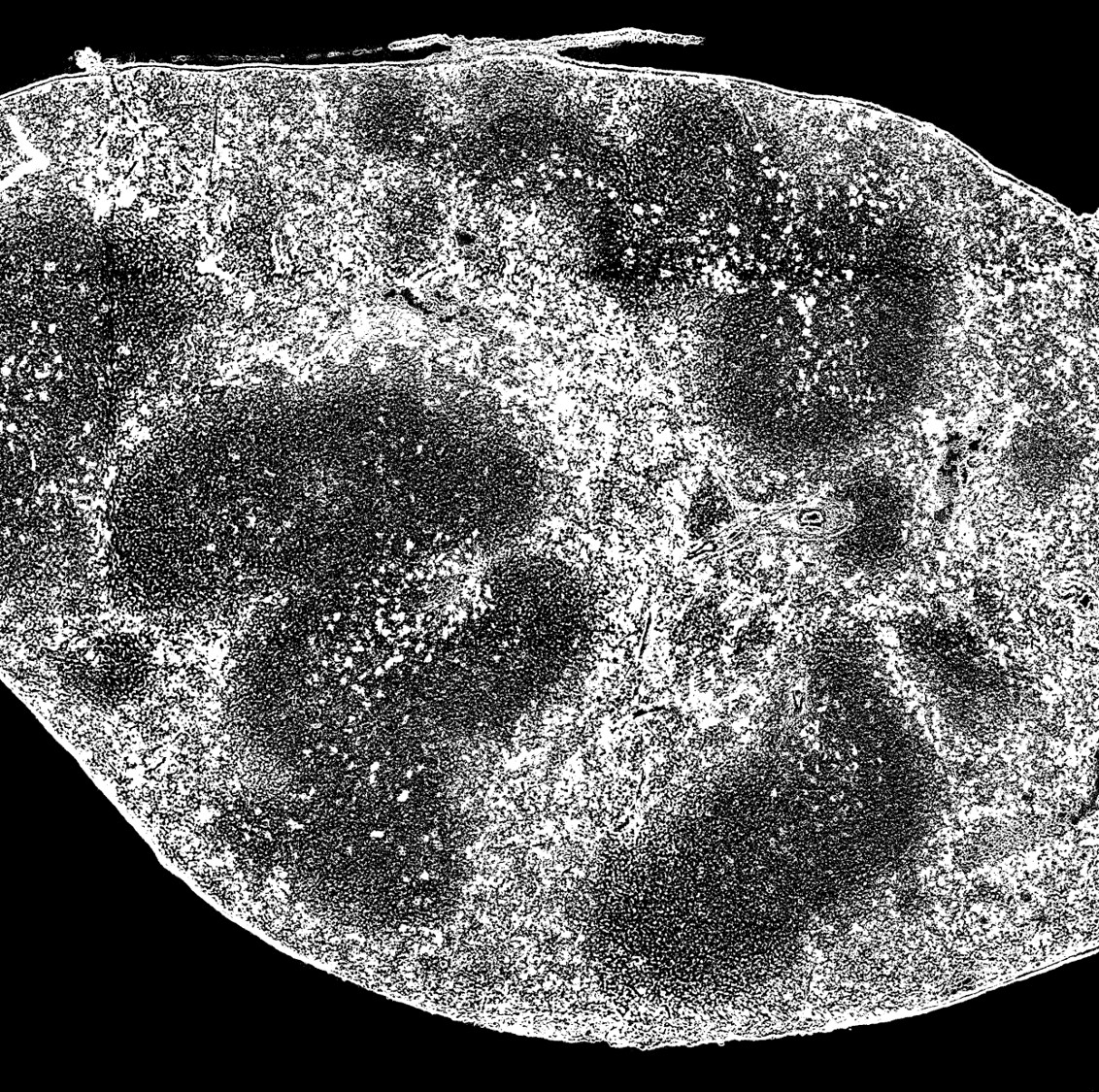
Use threashold function under Image->adjustment menu to adjust the image, so that your tissue is black and background is compeletely white.
Invert the color of the image. The final image is like "FFPE-2_BW.jpg" in the Example_Data folder.

Run the matlab script and a postion.txt file will be generated, which contains only the useful pixels.

Data visualization

The data visualization were completed with R language. The package used extensively the functions in Seurat V3.0 and ggplot2.

Common data visualization scripts include:

#For RNA:

No1_Prerun.R: count the RNA and UMI counts per pixel

No2_repair_filtered_matrix.R: remove the pixels not on tissue and correct for channels with defects

No3_Total_transcripts and Gene_count_after_correction.R: replot the RNA and UMI counts heatmap

No4_clustering_SCT&CLR.R: clustering and spatial plot with SCTranscform or CLR normalization.

#For Protein:

No1-No5 same as RNA script above.

No5_Individual gene plot_SCT&CLR.R: plot individual protein heatmap.

##Tissue images_manuscript

this folder contains all the microscope images in this manuscript.

Contact

For questions, you can contact Yang Liu (edicliuyang@gmail.com)