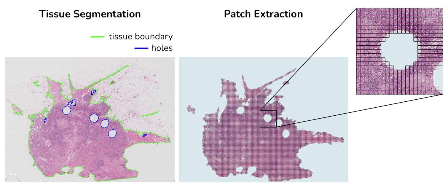
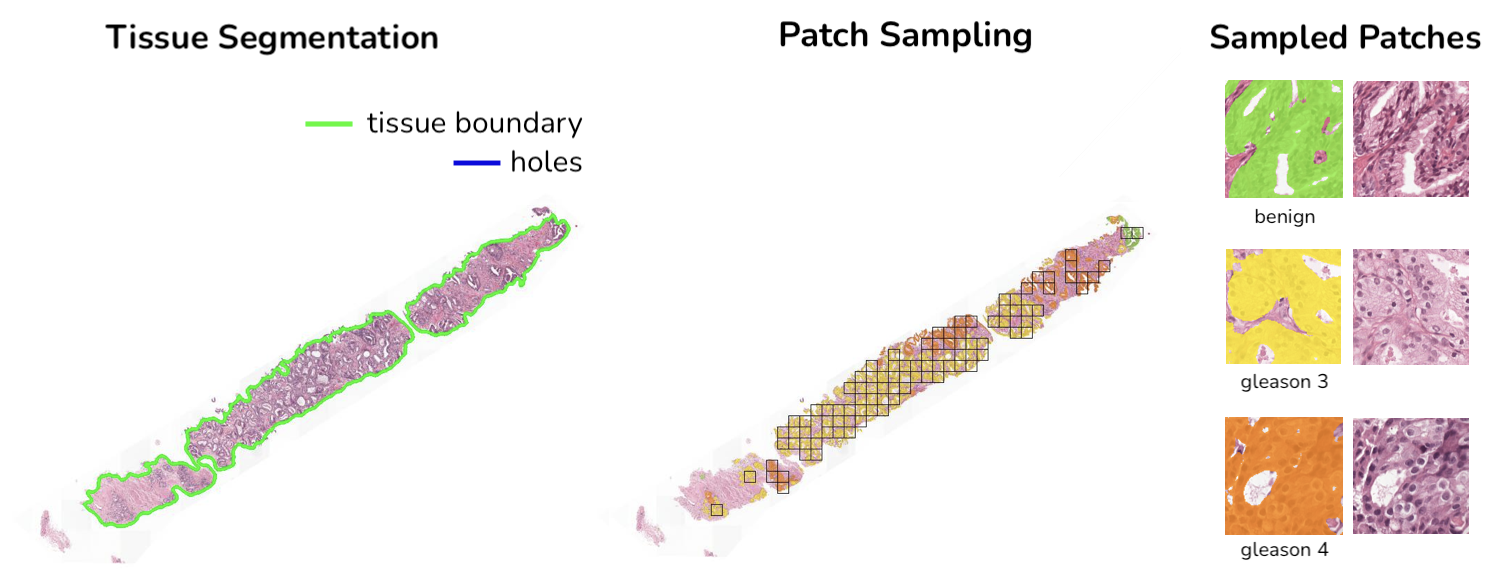
Histopathology Slide Pre-processing Pipeline

HS2P is an open-source project largely based on CLAM tissue segmentation and patching code.

Requirements

install requirements via pip3 install -r requirements.txt

Patch Extraction: Step-by-step guide

[Optional] Configure wandb

If you want to benefit from wandb logging, you need to follow these simple steps:

grab your wandb API key under your profile and export
run the following command in your terminal: export WANDB_API_KEY=<your_personal_key>
change wandb paramters in the configuration file under config/ (set enable to True)

Create a .csv file containing paths to the desired slides:

slide_id,slide_path
slide_id_1,path/to/slide_1.tif
slide_id_2,path/to/slide_2.tif
...

You can optionally provide paths to pre-computed segmentation masks under the 'segmentation_mask_path' column

slide_id,slide_path,segmentation_mask_path
slide_id_1,path/to/slide_1.tif,path/to/slide_1_mask.tif
slide_id_2,path/to/slide_2.tif,path/to/slide_2_mask.tif
...

Create a configuration file under config/extraction/

A good starting point is to use the default configuration file config/extraction/default.yaml where parameters are documented.

Run the following command to kick off the algorithm:

python3 patch_extraction.py --config-name <config_filename>

Depending on which flags have been set to True, it will produce (part of) the following results:

Patch extraction output

hs2p/
├── output/<experiment_name>/
│     ├── masks/
│     │     ├── slide_id_1.jpg
│     │     ├── slide_id_2.jpg
│     │     └── ...
│     ├── patches/<patch_size>/<format>/
│     │     ├── slide_id_1/
│     │     │     ├── slide_id_1.h5
│     │     │     └── imgs/
│     │     │         ├── x0_y0.<format>
│     │     │         ├── x1_y0.<format>
│     │     │         └── ...
│     │     ├── slide_id_2/
│     │     └── ...
│     ├── visualization/
│     │     └── <patch_size>/
│     │         ├── slide_id_1.jpg
│     │         ├── slide_id_2.jpg
│     │         └── ...
│     ├── tiles.csv
│     └── process_list.csv

masks/ will contain a downsampled view of the slide with tissue segmentation overlayed
visualization/ will contain a downsampled view of the slide where extracted patches are highlighted

tiles.csv contain patching information for each slide that ended up having patches extracted:

slide_id,tile_size,spacing,level,level_dim,x,y,contour
slide_id_1,2048,0.5,0,"(10496, 20992)",752,5840,0
...

Extracted patches will be saved as x_y.jpg where x and y represent the true location in the slide at level 0:

if spacing at level 0 is 0.25 and you extract [256, 256] patches at spacing 0.25, two consecutive patches will be distant from 256 pixels (either along x or y axis)
if spacing at level 0 is 0.25 and you extract [256, 256] patches at spacing 0.5, two consecutive patches will be distant from 512 pixels (either along x or y axis)

Patch Sampling: Step-by-step guide

[Optional] Configure wandb

see above

Create a .csv file containing paths to the desired slides & associated annotation masks:

slide_id,slide_path,annotation_mask_path
slide_id_1,path/to/slide_1.tif,path/to/slide_1_annot_mask.tif
slide_id_2,path/to/slide_2.tif,path/to/slide_2_annot_mask.tif
...

In the same way as for patch extraction, you can optionally provide paths to pre-computed segmentation masks under the 'segmentation_mask_path' column.

Create a configuration file under config/sampling/

A good starting point is to use the default configuration file config/sampling/default.yaml where parameters are documented.

Run the following command to kick off the algorithm:

python3 patch_sampling.py --config-name <config_filename>

Depending on your config, it will produce (part of) the following results:

Patch sampling output

hs2p/
├── output/<experiment_name>/
│     ├── annotation_mask/
│     │     ├── slide_id_1.jpg
│     │     ├── slide_id_2.jpg
│     │     └── ...
│     ├── segmentation_mask/
│     │     ├── slide_id_1.jpg
│     │     ├── slide_id_2.jpg
│     │     └── ...
│     ├── patches/
│     │     ├── raw/
│     │     │     ├── category_1/
│     │     │     │   ├── slide_id_1_x0_y0.<format>
│     │     │     │   ├── slide_id_1_x1_y0.<format>
│     │     │     │   └── ...
│     │     │     ├── category_2/
│     │     │     └── ...
│     │     ├── mask/
│     │     │     ├── category_1/
│     │     │     │   ├── slide_id_1_x0_y0_mask.<format>
│     │     │     │   ├── slide_id_1_x1_y0_mask.<format>
│     │     │     │   └── ...
│     │     │     ├── category_2/
│     │     │     └── ...
│     │     └── h5/
│     │           ├── slide_id_1.h5
│     │           ├── slide_id_2.h5
│     │           └── ...
│     ├── visualization/
│     │     ├── slide_id_1.jpg
│     │     ├── slide_id_2.jpg
│     │     └── ...
│     └── sampled_tiles.csv

annotation_mask/ will contain a downsampled view of the slide with corresponding annotation mask overlayed
segmentation_mask/ will contain a downsampled view of the slide with tissue segmentation overlayed
visualization/ will contain a downsampled view of the slide where sampled patches are highlighted

sampled_patches.csv contain information for each patch that ended up being extracted:

slide_id,category,x,y,pct
slide_id_1,category_1,3488,2512,0.8203125
...

Again, extracted patches will be saved as x_y.jpg where x and y represent the true location in the slide at level 0.

Resuming experiment after crash / bug

If, for some reason, the experiment crashes, you should be able to resume from last processed slide simply by turning the resume parameter in your config file to True, keeping all other parameters unchanged.

Troubleshooting

If the generated visualization are noisy, you'll need to change libpixman version. Running the following command should fix this issue: