In this project we detect the lane lines under more challenging real conditions, including lane cruvatures, change of lighting and lane colors, shadows, and different road conditions.
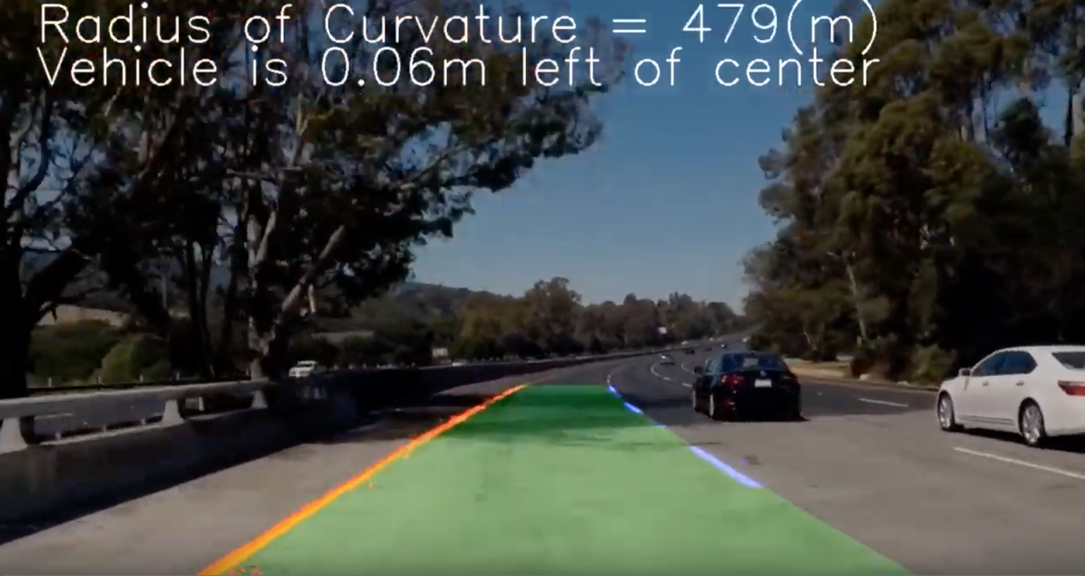
The input is camera videos of a vechicle driving on a highway and the output is the video annotated with and overlay that shows the detected lane, as well as detected readius of curvatures and the vehicle offset from center of the lane.
For each frame in the input video the steps of a pipeline is are applied including image processing, detection of the lanes, and estimation of lane curvature. The result of the pipeline is overlaid back on the original image.
Steps:
- Camera calibration
- Distortionn correction
- Gradient and color thersholding
- Perspective transform to rectify the image
- Detecting lane pixels and fitting a polynomial
- Detemining lane curvature and vehicle offset
- Warping detected lane boudaries back to the original image
- Visualizing lane boudaries and outputing lane curvature and vehicle offset
The images for camera calibration are stored in the folder called camera_cal. The images in test_images are result of testing the pipeline on single frames. The resulting imaages from each stage of the pipeline are stored in the folder called output_images.
The pipeline is then applied to the project_video.mp4 and the output is project_video_output.mp4
I will also test the pipeline on challenge_video.mp4 and the harder_challenge.mp4 video.
The code for this step is contained in the second code cell of the IPython notebook located in ./P2_Advanced_Lane_Finding.ipynb (or in lines 105 through 178 of the file P2_Advanced_Lane_Finding.py).
The function get_objpts(pattern_size) generates the 3D object points for a given pattern size. The pattern size is a tuple (nx, ny) for the number of corners in a chessboard calibration image pattern.
The camera_calibration() function gets a list of paths of calibration images and the pattern size. For each calibration image, it finds the chessboard corners using cv2.findChessboardCorners() function of OpenCV. If detection of chessboard corners is successful, the detected corners are added to the img_points list. For each image, a set of generated object points is also added to the obj_points list. After all calibration images are processed, the cv2.calibrateCamera() function of OpenCV is called with the image and object points to obtain the camera matrix and distortion coefficients.
The camera calibration step is only performed once at the beginning of the project. If it fails, the execution is stoped with a RuntimeException.
The function correct_distortion() gets a distorted image and the distortion coefficients and returns the undistorted image. An example of the undistorted calibration image is given below.
The first step of the pipeline is undistort the input frame. The obtained distortion coefficients are used to undistort every single frame of the video before it is further processed.
An example of undistorted frame from the test images is shown below. Pay attention to the difference in location of the white car in the original and undistorted image:
Gradient and color thresholding is applied to every undistorted frame to obtain the a binary image. The the threshold values are tuned so that that lane lines are distinct in the binary image.
Gradient thresholding is implemented in cell 4 of the notebook (or lines 181-245 in exported .py file). For gradient thresholding Sobel operator is applied in x and y direction. Also the magnitude and direction of the gradient is calculated. The final gradient threshold is a combination of all thresholds. Following figure shows the result of the combined gradient threshold on a test image.
For color thresholding (cell 5 in notebook, lines 247-273 in .py file) the image is first converted to HLS format. A Saturation and Hue thresholds are then implemented. The Hue threshold did not return good results of test images though.
Finally, a combination of gradient and saturation thresholds is applied to each input frame. This is implemented in the function apply_threshold() (cell 7 in notebook; lines 275-300 in Python file). The result of the combined gradient and color thresholding is shown in figure below. The left image shows the effect of gradient (green) and saturation (blue) thresholds. The right image shows the result of applying the combined binary threshold to the input frame.
To detect the road curvature the image must be changed to bird eye perspective.
The code for obtaining the perspective transform matrix and warping the images is implemented in cell 6 in the notebook (lines 304-355 in the Python file).
The get_warp_matrix() function returns the warp matrix for rectifying a camera frame and its inverse. The assumption is that an isosceles trapezoid will be warped into a rectangle. The trapezoid is centered on the image. The input parameters image_size, top_y, top_width, and bottom_width define the trapezoid. The default values for the input parameters were determined by checking multiple images of the straight roads. The warp matrix is only needs to be calculated once.
The function rectify() then takes the warp matrix to transform every input frame to the bird eye view.
The figure below shows the points defining the trapezoid on an image of straight road (left) and the warped frame (right). As can be seen, the warp matrix effectively transforms the straight road lane lines into vertical parallel lines in the bird eye image.
Figure below shows the warped binary image for the test image with a curve.
The function find_lanes_sliding_window() in 8th code cell in the notebook (lines 360-483 in Python file) performs a sliding window algorithm on the input binary rectified image and returns the (y, x) coordinate of pixels belonging to each left and right lanes. This function also returns the offset of lane midpoint from image midpoint in pixels.
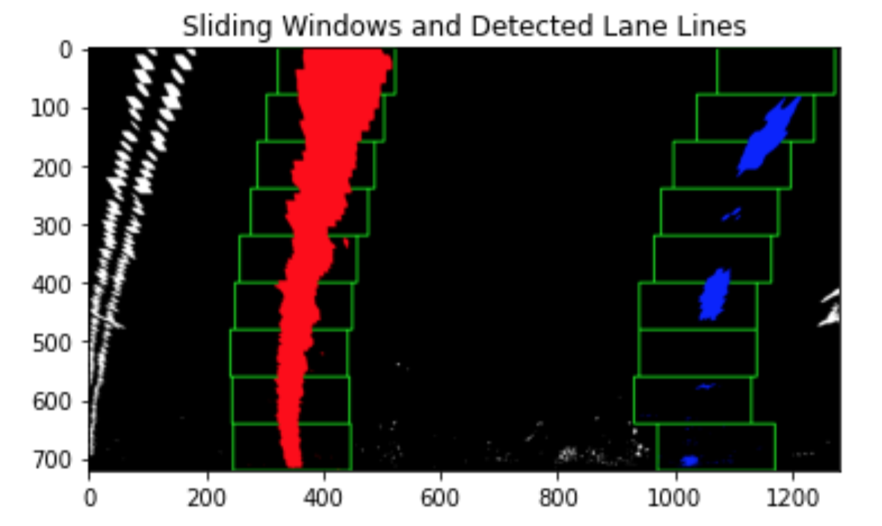
From the input binary warped image, the base of the lanes are detected using peaks of a histogram. Using the bases the boundaries of the sliding windows are determined. For each window, for the left and right lane line, the function then finds the x and y coordinates of the nonzero binary activations and adds them to the corresponding list for the lane pixels. Following figure shows the sliding windows and the detected pixels for each lane:

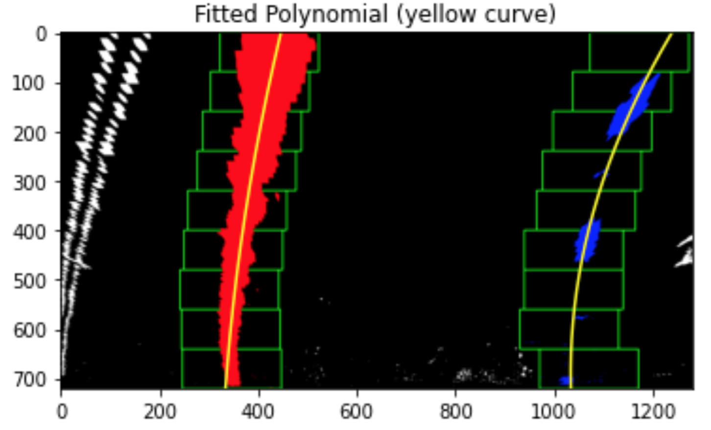
The detected lane line pixels are used to fit a 2nd order polynomial for the curve using numpy's polyfit() function in 9th code cell in the notebook (lines 486-535 in Python file). The result is shown below for the test image:
Calculating the radius of curvature of the lane and the position of the vehicle with respect to center
After the 2nd order polynomial is found for the lane lines, the curvature of each lane line is estimated in the eval_lane_curvature() method in 10th code cell of the notebook (lines 538-593 in Python file).
The coefficients of the fitted polynomials are in pixels. Accordingly the calculated curvature would be also in pixels. In order to get the curvature in meters, the coefficients of the left and right polynomial are first converted to meters using my and mx scale factors for the y and x directions. The scale factors are in meters per pixel units. The converted coefficients are then used to calculate and return the curvature for the left and right lane lines in meters. The function also returns the direction of the curvature (right curve, left curve, or straight road).
The function eval_vehicle_offset() gets the offset of the midpoint of the lanes from the middle of the image as input. Using the scale factor (meters per pixel) for x direction it calculates the offset of the vehicle from middle of the lane. It also return the direction of the offset (right, if offset is positive, and left if offset is negative).
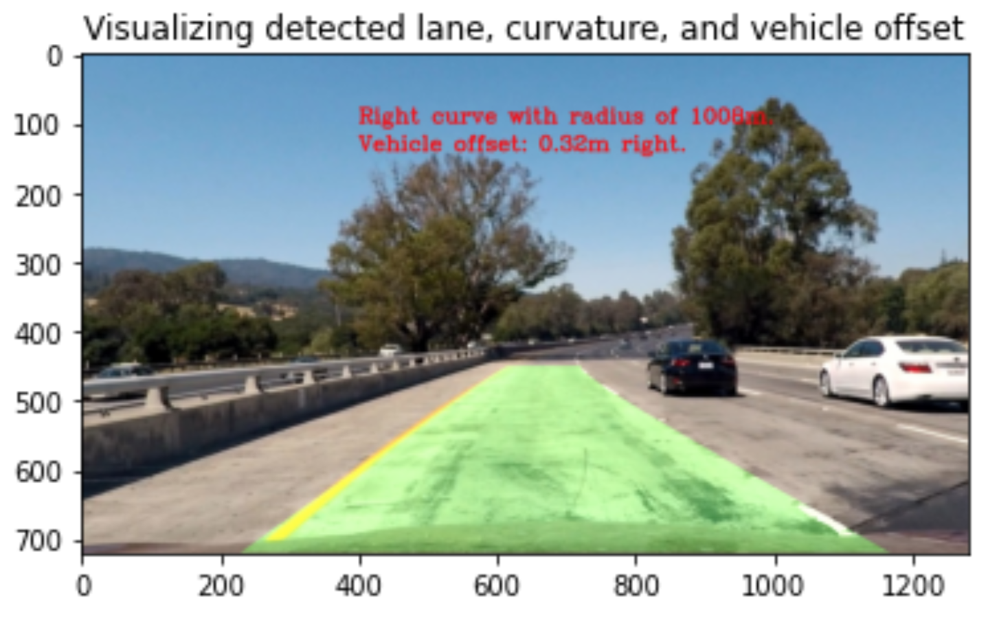
Finally the functions visualize_lane() and visualize_info() in the 11th code cell in the notebook (lines 616-683 in the Python file) visualize the detected lane, the radius of the lane curvature, and the offset of the vehicle form middle of the lane. An example is shown below:
For displaying the curvature, the average from curvature of the left and right lane lines is shown.
Here's a link to my video result
Due to time reasons I only focused on first implementing the requirements of the project rubric. Specifically, my code lacks the following points which would improve the performance and robustness of the algorithm:
- I am not using a Line class to keep track of the detected lines, and the results of previous frames.
- I didn't apply the search ahead algorithm to detect the lines from the previous results, instead of running the sliding window on every frame
- I am not checking for too sharp curves that would go out of the left or right side of the image.
- I am not applying smoothing to compensate for outliers.
All above points could contributed significantly to the performance and robustness of the algorithm.
Another important point is the thresholding. I use global values for thresholds for all the frames. The project_video.mp4 has a very good lighting condition and contrast between road and the lane lines, which allows this thresholding approach still work well. In comparison global threshold values does not work on more challenging lighting and contrast situations like challenge_video.mp4 and harder_challenge_video.mp4.
To summarize, to pursue more on this project, I would first implement the above points to improve the overall performance and robustness of the algorithm. I would then try other thresholding approaches (like adaptive thresholding) and different combinations of thresholds in order to get better results for the challenge videos.


