deepsea-keras

Keras implementation of DeepSEA, original version published in Nature Methods 2015 here.

Updates

May 6, 2020: wrap into a package for re-use (especially on reading data)

Setup

After cloned the Github repository, initialize a new Anaconda environment using the conda_env.yml configurations.

Build Model

First download the compiled dataset from DeepSEA official site here: http://deepsea.princeton.edu/help/

Put the download *.mat files under ./data/ folder.

For the trained parameters file, download from sourceforge: https://sourceforge.net/projects/bionas/files/DeepSEA_v0.9/

Now there are two different routes to go:

if loading from the original torch parameters: download deepsea_cpu.pth to data folder, then open python terminal:

from load_torch_weights import build_and_load_weights
model = build_and_load_weights()

Note: This file is a torch7 file with all trained parameters in an OrderedDict python object, when loaded with torch.load method.

The t7 file can be downloaded here

if loading from the converted Keras model, download the Keras parameter file:

from model import load_model
model = load_model()

The keras h5 file can be downloaded here.

Prediction

Make sure we did not do anything crazy; the results should be the same regardless of which model building route you took:

from evaluate import val_performance
import numpy as np
val_evals = val_performance(model)
print(np.nanmean(val_evals['auroc'])) # 0.937
print(np.nanmean(val_evals['aupr']))  # 0.402

Also we can evaluate the test-data performance. This might take a bit longer using a single GPU, so we can convert the Keras model to a Multi-GPU model:

Note: Remember to toggle the gpus argument to the available gpus you have.

from evaluate import test_performance
from model import convert_to_multigpu
mg_model = convert_to_multigpu(model, gpus=3)
test_evals = test_performance(mg_model)
print(np.nanmean(test_evals['auroc'])) # 0.931
print(np.nanmean(test_evals['aupr']))  # 0.338

The results should be close enough to "average AUC of 0.933 and AUPRC of 0.342", as stated in the Selene biorxiv manuscript at the bottom of Page 5.

Explore

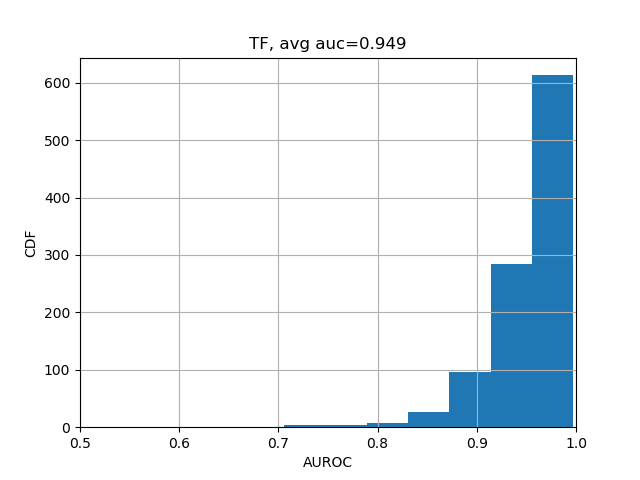
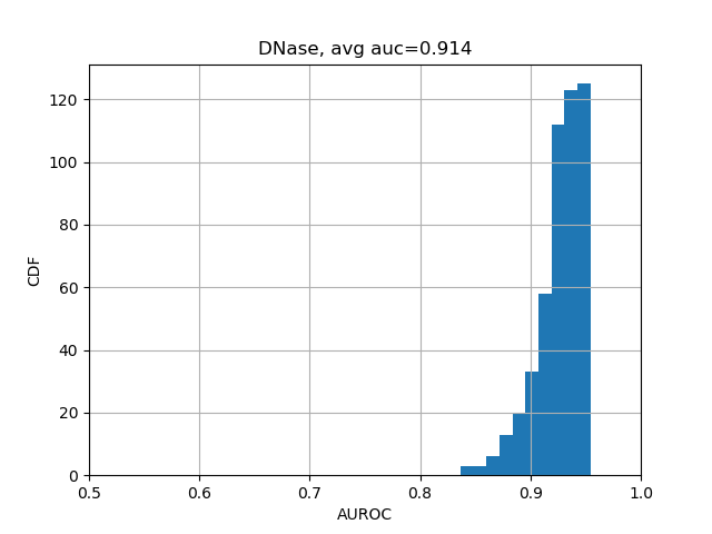
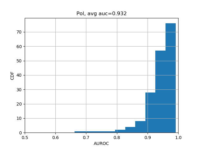
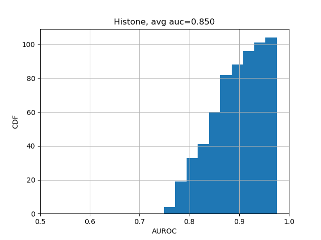
We can further break down the prediction accuracies by their categories:

from plot import plot_auc
plot_auc(test_evals)

The results should look like the following

zj-zhang/deepsea_keras