sc-power-analysis

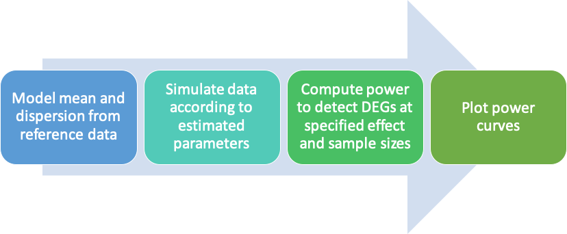
A snakemake pipeline for scRNA-seq power analyses.

Introduction

This pipeline estimates power to detect differentially expressed genes from scRNA-seq data at various numbers of samples/cells and effect sizes. It models mean and dispersion parameters on a Negative Binomial distribution from reference data and simulates representative UMI count data from these estimates. The user can define various simulation parameters, such as the number of differentially expressed genes, effect sizes, number of samples, and number of cells.

Parameter estimation on reference data

Given a reference count matrix, we fit the observed counts for each gene to a Negative Binomial distribution and estimates the mean and dispersion parameters. Our likelihood function includes a scaling factor for the mean equivalent to the sequencing depth of each cell.

Data simulation

For each replicate, we generate a simulated count matrix reflecting a total number of genes and cells specified in the inputs. We simulate data for a control condition and a treatment condition. To begin, we randomly sample from the observed sequencing depths to generate a vector of scaling factors equivalent in size to the number of cells specified for the simulation. For each gene, we randomly sample a mean and dispersion parameter (with replacement) from the estimated parameters in the previous step and randomly sample from the Negative Binomial distribution defined by these parameters (with sequencing depth-scaled mean) to simulate the observed counts for this gene. The same mean and dispersion parameter are used for each gene across the control and treatment conditions. For a set of ground truth DEGs, we multiply the mean parameter used in the control condition by an effect size to simulate the gene's expression in the treatment condition.

DGE testing and power analysis

We use Seurat's FindMarkers() function to test for DEGs (after normalizing the simulated count data with Seurat). The user may specify the test to use, but we have found that the wilcox option works best based on power for DEG detection and runtime. We then compute the power based on the Bonferroni-corrected p-values of the results. After computing the power at each sample size and effect size specified, we plot the power curves and return a plot in .pdf format.

Download

Clone the repository to your desired destination.

git clone https://github.com/zrcjessica/sc-power-analysis.git

Dependencies

This pipeline was written with snakemake version 5.20.1. We recommend that you follow these instructions for snakemake installation via conda. This will install snakemake in an isolated environment, which is the recommended best practice for avoiding package conflicts. This allows you to use the --use-conda flag when running the pipeline, which will automatically install the package specified in the environment.yml file. If you do not install snakemake in an isolated environment, then make sure you have installed all of the conda packages listed in environment.yml.

Inputs

All input parameters are defined in the config.yml file and must be edited accordingly to suit your own data.

`data`

The data variable in the config.yml file contains the names of all samples for which you have count data available. Each sample name also stores the paths to the count matrix files under counts variable.

This pipeline is designed to take UMI count matrices in compressed Matrix Market format (*.mtx.gz). We suggest using the matrix.mtx.gz file associated with the filtered feature-barcode matrix from Cell Ranger.

Example:

data:
  SampleA:
    counts: data/SampleA/outs/filtered_feature_bc_matrix/matrix.mtx.gz
  Sample B:
    counts: data/SampleB/outs/filtered_feature_bc_matrix/matrix.mtx.gz
  Sample C:
    counts: data/SampleC/outs/filtered_feature_bc_matrix/matrix.mtx.gz

`sample`

Include the name(s) of the sample you want to use as reference panel(s) for your power analyses. Each power analysis takes one reference panel as input. If you choose to include a list of samples here, then the pipeline will return a plot of power curves for each sample.

Example:

sample: SampleA

`params`

Input parameters to the simulation are described here.

replicates: the number of replicates to include in the power analysis. Can be a list of integers or a single fixed value.
cells: the number of cells to include in the power analysis. Can be a list of integers or a single fixed value.
effects: a list of the effect sizes to include in the power analysis.
alpha: the significance level to use for DGE testing.
nGenes: number of genes in each simulated count matrix.
pctDegs: percent of nGenes to be simulated as DEGs.
nSims: number of simulations for each power analysis calculation.
test: test to use for DGE testing; from list of options for the test.use argument in Seurat's FindMarkers() function. wilcox is recommended.
sample_variable: one of replicates or cells. Specifies the value to be plotted on the x-axis of the power curve plot. The variable specified here must be defined by a list of values.

Example:

params:
  replicates: [1,3,5,7,10]
  cells: 5000
  effects: [1.25, 1.5, 1.75, 2]
  alpha: 0.05
  nGenes: 10000
  pctDegs: 0.05
  nSims: 15
  test: wilcox
  sample_variable: replicates

`out`

Path to directory to save output files.

Example:

out: out

Output

This pipeline returns a table of power estimations at each effect size and sample size specified in config.yml and a plot of power curves.

Execution

You can run this pipeline locally with

./run &

These computations take a long time, so we encourage the use of a compute cluster. This pipeline supports Sun Grid Engine. Run the pipeline on an SGE cluster with:

qsub run